Using variables in the `design` argument of `TVGEV`

Using variables in the `design` argument

The design argument of the TVGEV function is intended to be “language”. It can embed a “parameter” given as a R object in the environment, yet this can cause problems due to the scoping rules, especially when the TVGEV function is used from within a function.

Example change of slope in a broken line trend

As an example, we will consider the case where a time trend is specified as a broken line with a slope zero before the time of change say $u$ and an unknown slope after the time $u$ . This is similar to a kink regression in the linear regression framework.

It is not possible with NSGEV to consider $u$ as a model parameter because TVGEV models are assumed to link each of the three GEV parameters to a linear predictor having the form $\mathbf{x}(t)^\top \boldsymbol{\psi}$ . Incidentally, would $u$ be considered as a model parameter, the log-likelihood would no longer be differentiable w.r.t. $u$ , and adjustments would be required in the likelihood-based inference. However we can think of using a grid of candidate values for the change of slope time $u$ : by fitting the model with $u$ fixed to each grid value say $u_i$ for $i=1$ , $2$ , … we can compute the corresponding maximised log-likelihoods and then choose the value of $u$ as the grid value with maximal log-likelihood. It is convenient to write a function inside which the loop on the candidate values is found. The broken line can be obtained with the breaksX design function: the breaks argument correspond to the knots of truncated power splines. By using a single knot one gets two basis functions (see the help for breaksX). One only needs to use the broken line basis function with name t_1990 if for example the change of slope $u$ is located at year 1990. A possible problem arises from the fact that the candidate value $u_i$ has to be passed to the design function.

For illustration, consider the Dijon_TXmax example: assume that the plausible breaks are in the range 1970 to 2000. To make things slightly more general we assume that col contains the name of the column for the maxima in the data frame maxData.

fitBreaks <- function(maxData, col) {   
    if (!inherits(maxData$year, "Date")) {
        maxData$year <- as.Date(paste0(maxData$year, "-01-01"))
    }
    res <- desCall <- list()
    yearBreaks <- c(1970:2000)
    for (ib in seq_along(yearBreaks)) {
        if (TRUE) { ## WORKS 
            desCall[[ib]] <-
                sprintf("breaksX(date = year, breaks = \"%4d-01-01\", degree = 1)",
                        yearBreaks[ib])
            floc <- sprintf("~ t1_%4d", yearBreaks[ib])
            text <-
                sprintf(paste0("TVGEV(data = maxData, response = col, date = \"year\",\n",
                               "       design = %s,\n",
                               "      loc = %s)\n"),
                        desCall[[ib]], floc)
            res[[ib]] <- eval(parse(text = text))
        } else { ## DOES NOT WORK
            d <- sprintf("%4d-01-01", yearBreaks[ib])
            floc <- sprintf("~ t1_%4d", yearBreaks[ib])
            res[[ib]] <- TVGEV(data = maxData, response = col, date = "year",
                               design = breaksX(date = year, breaks = d, degree = 1),
                               loc = floc)
        }
    }
    ll <- sapply(res, logLik)
    iMax <- which.max(ll)
    ## Compute lims to include the 'confidence' logLik level
    llLim <- ll[iMax] - qchisq(0.95, df = 1) / 2
    yearMax <- yearBreaks[iMax]
    plot(yearBreaks, ll, type = "o", pch = 21, col = "orangered",
         ylim = range(ll, llLim)                               ,
         lwd = 2, bg = "gold", xlab = "break", ylab = "log-lik")
    grid()
    iMax <- which.max(ll)
    abline(v = yearMax)
    abline(h = ll[iMax] - c(0, qchisq(0.95, df = 1) /2),
           col = "SpringGreen3", lwd = 2)
    fit <- res[[iMax]]
    return(fit)  
}

names(TXMax_Dijon) <- c("year", "TXMax") 
(fitL <- fitBreaks(maxData = TXMax_Dijon, col = "TXMax"))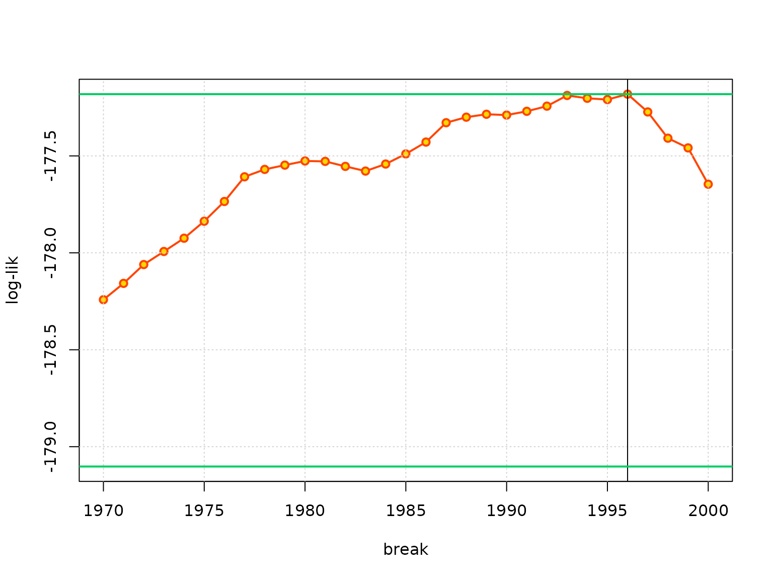

## Call:
## TVGEV(data = maxData, date = "year", response = col, design = breaksX(date = year, 
##     breaks = "1996-01-01", degree = 1), loc = ~t1_1996)
## 
## Coefficients:
##              Estimate Std. Error
## mu_0       32.6483420 0.23098848
## mu_t1_1996  0.1328950 0.03771828
## sigma_0     1.7427827 0.14585534
## xi_0       -0.1704297 0.07243566
## 
## Negative log-likelihood:
## 177.181

Explanation

The object given in the design formal argument is normally a call to a function, which is internally used with do.call. If a R object such as d is used in the call, it is first looked for in the environment of the call (here, the data frame), then in the environment of the function (hre, fitbreaks). In both cases d does not exist.

We could turn d into a (constant) column of the data fame: this would make the estimation successful. Yet the fitted object would require for a prediction with oredict that the column d is found in the provided new data, which is tedious. The solution chosen here is to parse a code with the variables replaced by their value. We see that the returned TVGEV object contains the wanted formula and the wanted design. It does no longer relate to an extra R variable.

From a statistical perspective, it must be kept in mind that the ML estimate of the break does not have the standard normal distribution, because the log-likelihood function is not differentiable. On intuitive grounds, the estimate should be “super-efficient”. Using the classical chi-square approximation to derive a profile likelihood interval should consequently lead to an interval with a coverage rate that is larger than the nominal one. On the plot the horizontal green lines show the maximised log-likelihood $\ell_{\texttt{max}}$ and the value $\ell_{\texttt{max}} - \delta$ that would be used to find the limits of a profile likelihood confidence interval under the classical regularity conditions, which are not met here.

Yves Deville deville.yves@alpestat.com and Nathan Bengaouer nath.bengaouer@asnr.fr

2026-02-25