The broken line trend
In this report we simulate a trend for the location parameter. We chose the model with constant scale and shape , while the location is given by
where the annual block
is chosen to be
,
and the data will from 1921 to 2020. Using the breaksX
design function we get a matrix X with a linear trend
t1 and a broken line t1_1980 with slope:
before 1980 and slope
from
on.
library(NSGEV)
date <- as.Date(sprintf("%4d-01-01", 1921:2020))
X <- breaksX(date = date, breaks = "1980-01-01")
rownames(X) <- format(date, "%Y")
n <- nrow(X)
plot(date, X[ , 1], ylim = range(X), type = "n", xlab = "", ylab = "")
matlines(date, X, type = "l", lwd = 2) 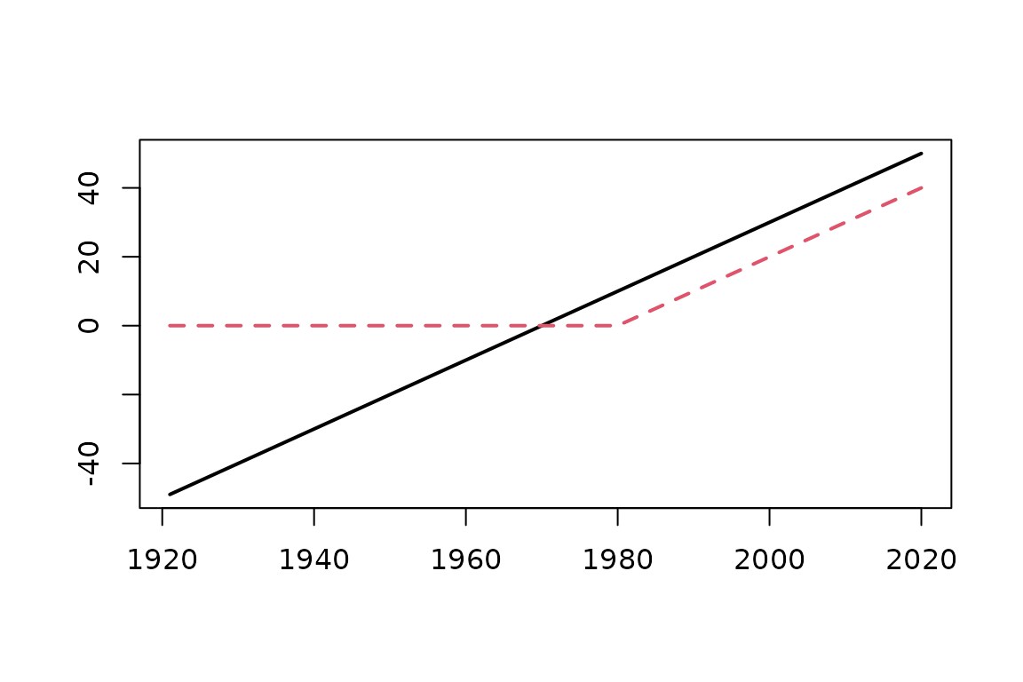
Simulation of the data and GEV estimation
We simulate a sample of size ns for the vector
of
coefficients
,
,
and
.
The results are stored in a matrix psi with ns
rows.
set.seed(1234)
GEVnms <- c("loc", "scale", "shape")
ns <- 400
pLoc <- 3
psiLoc <- matrix(rnorm(ns * pLoc, sd = 0.15), nrow = ns)
sigma <- rgamma(ns, shape = 4, rate = 2)
xi <- rnorm(ns, sd = 0.1)
psi <- cbind(psiLoc, sigma, xi)
colnames(psi) <- c(paste("mu", c("0", colnames(X)), sep = "_"), "sigma_0", "xi_0")
p <- ncol(psi)
kable(head(psi, n = 4), digits = 3)| mu_0 | mu_t1 | mu_t1_1980 | sigma_0 | xi_0 |
|---|---|---|---|---|
| -0.181 | -0.184 | -0.154 | 0.684 | -0.047 |
| 0.042 | 0.005 | -0.208 | 1.247 | 0.058 |
| 0.163 | -0.063 | -0.007 | 0.608 | 0.042 |
| -0.352 | -0.135 | 0.272 | 3.302 | 0.068 |
Then we create a three-dimensional array theta with
dimension c(ns, n , 3). A slice theta[is, , ]
will contain the GEV parameters for the simulation number
is i.e., a matrix with dimension c(n , 3) of
the GEV parameters
for the blocks
to
.
theta <- array(NA, dim = c(ns, n, 3), dimnames = list(NULL, rownames(X), GEVnms))
Y <- mu <- array(NA, dim = c(ns, n), dimnames = list(NULL, rownames(X)))
fitTVGEV <- fitextRemes <- fitismev <- list()
co <- array(NA, dim = c(ns, 3, p),
            dimnames = list(NULL, c("NSGEV", "extR", "ismev"), colnames(psi)))
ML <- array(NA, dim = c(ns, 3),
            dimnames = list(NULL, c("NSGEV", "extR", "ismev")))
CVG <- array(NA, dim = c(ns, 3),
             dimnames = list(NULL, c("NSGEV", "extR", "ismev")))
estim <- "optim"
for (is in 1:ns) {
    mu <- cbind(1, X) %*% psiLoc[is, ]
    theta[is, , ] <- cbind(mu, sigma[is], xi[is])
    Y[is, ] <- rGEV(1,
                    loc = theta[is, , 1],
                    scale = theta[is, , 2],
                    shape = theta[is, , 3])

    df <- data.frame(date = date, Y = Y[is, ])
    fitTVGEV[[is]] <- try(NSGEV::TVGEV(data = df, response = "Y", date = "date",
                                       design = breaksX(date = date,
                                           breaks = "1980-01-01",
                                           degree = 1),
                                       estim = estim,
                                       loc = ~ t1 + t1_1980))
    if (!inherits(fitTVGEV[[is]], "try-error")) {
        if (estim == "optim") {
            CVG[is, "NSGEV"] <- (fitTVGEV[[is]]$fit$convergence == 0)
        } else {
            CVG[is, "NSGEV"] <- (fitTVGEV[[is]]$fit$status > 0)
        }
        if (CVG[is, "NSGEV"]) {
            co[is, "NSGEV", ] <- coef(fitTVGEV[[is]])
            ML[is, "NSGEV"]  <- logLik(fitTVGEV[[is]])
        }
    } else CVG[is, "NSGEV"] <- FALSE

    df.extRemes <- cbind(df, breaksX(date = df$date, breaks = "1980-01-01",
                                     degree = 1));
    fitextRemes[[is]] <- try(extRemes::fevd(x = df.extRemes$Y, data = df.extRemes,
                                            loc = ~ t1 + t1_1980))
    if (!inherits(fitextRemes[[is]], "try-error")) {
        CVG[is, "extR"] <-  (fitextRemes[[is]]$results$convergence == 0)
        if (CVG[is, "extR"]) {
            co[is, "extR", ] <- fitextRemes[[is]]$results$par
            ML[is, "extR"] <-  -fitextRemes[[is]]$results$value
        }
    } else CVG[is, "extR"] <- FALSE
    fitismev[[is]] <- try(ismev::gev.fit(x = df.extRemes$Y,
                                         y = as.matrix(df.extRemes[ , c("t1", "t1_1980")]),
                                         mul = 1:2, show = FALSE))
    if (!inherits(fitismev[[is]], "try-error")) {
        CVG[is, "ismev"] <- (fitismev[[is]]$conv == 0)
        if (CVG[is, "ismev"]) {
            co[is, "ismev", ] <- fitismev[[is]]$mle
            ML[is, "ismev"] <-  -fitismev[[is]]$nllh
        }
    } else CVG[is, "ismev"] <- FALSE

}
Error in solve.default(xhessian) : Lapack routine dgesv: system is exactly singular: U[2,2] = 0
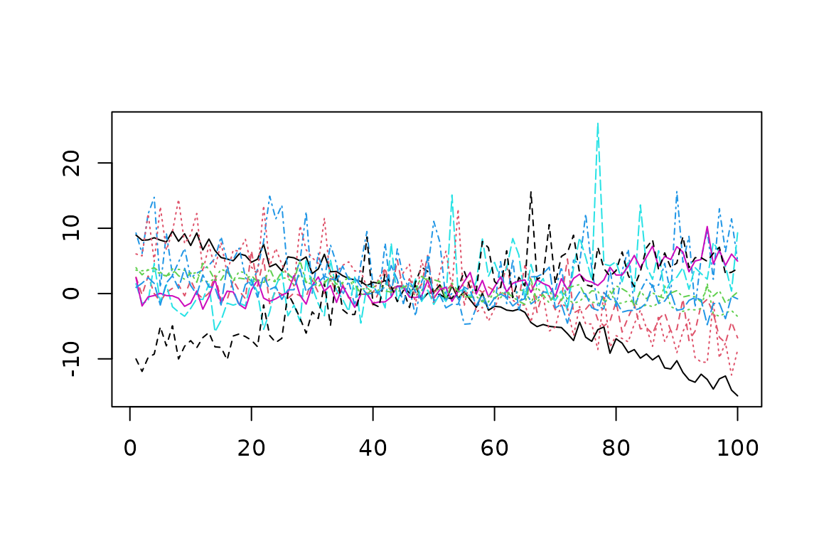
Ten simulated paths
Results
We can assess the convergence for the three estimation methods.
| NSGEV | extR | ismev |
|---|---|---|
| 400 | 399 | 394 |
We can inspect the content of the array co containing
the estimated coefficients
.
| NSGEV.1 | extR.1 | ismev.1 | NSGEV.2 | extR.2 | ismev.2 | NSGEV.3 | extR.3 | ismev.3 | |
|---|---|---|---|---|---|---|---|---|---|
| mu_0 | -0.236 | -3.070 | -3.396 | 0.174 | 0.174 | 0.174 | 0.095 | 0.095 | 0.095 |
| mu_t1 | -0.184 | -0.153 | -0.220 | 0.005 | 0.005 | 0.005 | -0.066 | -0.066 | -0.066 |
| mu_t1_1980 | -0.143 | -0.228 | -0.056 | -0.206 | -0.206 | -0.206 | 0.006 | 0.006 | 0.006 |
| sigma_0 | 0.728 | 6.612 | 6.090 | 1.317 | 1.317 | 1.317 | 0.560 | 0.560 | 0.559 |
| xi_0 | 0.010 | -1.030 | -1.116 | 0.136 | 0.136 | 0.136 | 0.089 | 0.089 | 0.089 |
There are cases where the estimation fails, and also cases where
estimations seem successful but lead to very different estimated
coefficients. In such case, we can compare the maximised log-likelihood
stored in the array ML. For example this happens here for
the first simulation; we selected the random seed so that the results
for first estimation differ, but the conclusion are the same when
another seed is used. The log-likelihoods for the four first simulated
samples are as follows.
| sim 1 | sim 2 | sim 3 | |
|---|---|---|---|
| NSGEV | -127.229 | -193.43 | -104.646 |
| extR | -224.028 | -193.43 | -104.646 |
| ismev | -217.656 | -193.43 | -104.646 |
so the estimation produced by NSGEV seems better for simulation , since it leads to a greater log-likelihood. Note the estimated shape parameter both with extRemes and ismev which can be considered as an alert. Indeed, as far as is allowed we could find an infinite log-likelihood and an estimated shape can be considered as a non-convergence or as an error.
We notice that both extRemes::fevd and
ismev::gev.fit tend to find not infrequently very low
values for the estimated shape,
.
xiRange <- apply(co[ , , "xi_0"], 2, range, na.rm = TRUE)
rownames(xiRange) <- c("shape min", "shape max")
kable(xiRange, digits = 3)| NSGEV | extR | ismev | |
|---|---|---|---|
| shape min | -0.518 | -1.301 | -1.558 |
| shape max | 0.428 | 0.428 | 1.073 |
In order to compare the maximised log-likelihoods for the two
packages, we will consider that these are nearly equal when their
absolute difference is
and set any NA value to -Inf
ML[is.na(ML)] <- -Inf
compML <- table(cut(ML[ , "NSGEV"] - ML[ , "extR"],
                    breaks = c(-Inf, -0.05, 0.05, Inf),
                    labels = c("NSGEV < extR",
                        "NSGEV ~ extR",
                        "NSGEV > extR")))
kable(t(compML))| NSGEV < extR | NSGEV ~ extR | NSGEV > extR |
|---|---|---|
| 0 | 381 | 19 |
plot(ML[ , c("NSGEV", "extR")], asp = 1, pch = 16, col = "orangered", cex = 0.8)
abline(a = 0, b = 1)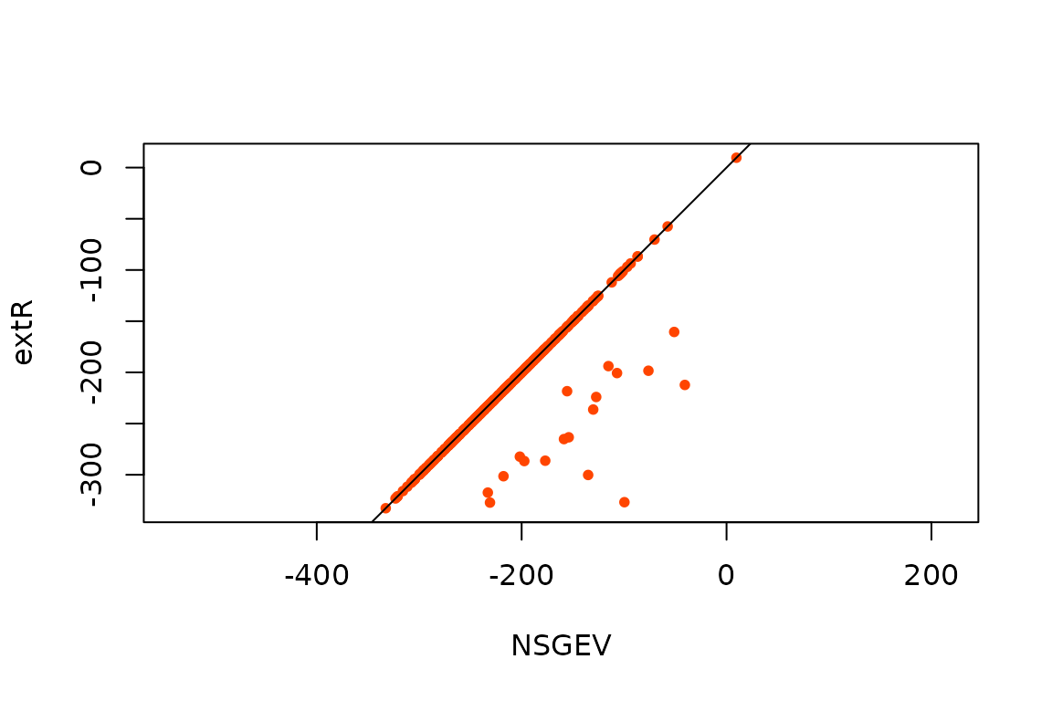
Comparison of the maximised log-likelihoods.
compML <- table(cut(ML[ , "NSGEV"] - ML[ , "ismev"],
                    breaks = c(-Inf, -0.05, 0.05, Inf),
                    labels = c("NSGEV < ismev",
                        "NSGEV ~ ismev",
                        "NSGEV > ismev")))
kable(t(compML))| NSGEV < ismev | NSGEV ~ ismev | NSGEV > ismev |
|---|---|---|
| 0 | 360 | 40 |
plot(ML[ , c("NSGEV", "ismev")], asp = 1, pch = 16, col = "SeaGreen", cex = 0.8)
abline(a = 0, b = 1)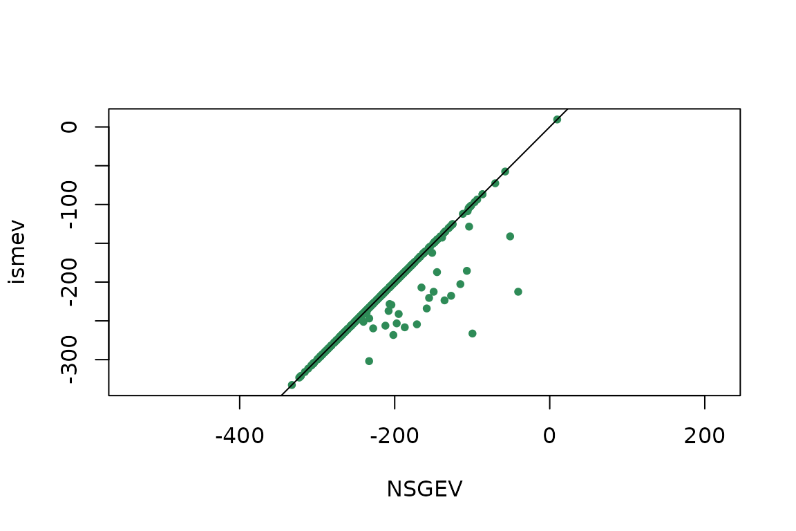
Comparison of the maximised log-likelihoods.
We find that for this kind of model, the maximised log-likelihood
found by NSGEV::TVGEV is comparable to that found by
extRemes::fevd and is even greater for a quite large
proportion of cases. More problems of convergence were found when using
the function ismev::gev.fit than when using the two other
functions.
As a possible explanation for the fact that NSGEV::TVGEV
performs better than the two other functions is that is uses better
initial values, based on linear regression. However this way of getting
initial values is straightforward only for models with constant scale
and shape as is the case here.
Findings
In this example, we find that for the kind of model studied here.
All of the three functions
NSGEV::TVGEV,extRemes::fevdandismev::gev.fitcan experiment problems of convergence. These problems are much more frequent withismev::gev.fitthan with the two other functions, and also seem to be pretty less frequent withNSGEV::TVGEVthan withextRemes::fevd.A problem with the functions
extRemes::fevdandismev::gev.fitis that they quite often find estimates with a shape which can be considered as absurd. For the simulated data used here, the risk of finding is higher when the linear trend is stronger, i.e. when the slope takes a larger absolute value. Since real data usually show a weaker dependence on the covariates than the data used here, the problems of convergence shown here have been overstated.