Time-Varying Models in NSGEV
Yves Deville
2026-04-15
Source:vignettes/IntroTVGEV.Rmd
IntroTVGEV.RmdThis document was created with NSGEV 0.2.3.
Scope
The NSGEV package provides a class of R objects
representing models for observations following a Time-Varying
Generalized Extreme Value (GEV) distribution, usually block maxima, as
described in the chapter 6 of the book by Coles (Coles 2001). This class of models is named
"TVGEV". These models are specific Non-Stationary GEV
models: only slowly varying functions of the time can be used as
covariates. They can be fitted by using CRAN packages such as
ismev (Rpack_ismev?),
evd (Stephenson 2002),
extRemes (Gilleland and Katz
2016) and more. However with these packages, the particularities
of the Time-Varying context are not taken into account, and it is quite
difficult for instance to compute predictions. The TVGEV
class and its methods have the following features.
Return levels are easily computed for a given time.
The inference on return levels can be obtained by profile-likelihood, using a dedicated algorithm.
The return level specific to the time-varying framework of Parey et al (Parey, Sylvie and Hoang, Thi Thu Huong and Dacunha-Castelle, Didier 2010) can be computed as well as profile-likelihood confidence intervals on it.
Graphical diagnostics favour the ggplot system (Wickham 2016). The
autoplotandautolayerS3 methods are consequently used instead of theplotandlinesS3 methods of the classical graphics package.
The present vignette shows how models can be specified and fitted, and illustrates the use of the principal methods.
A simple linear trend on the GEV location
Data for illustration
We begin by using the dataset TXMax_Dijon shipped with
the package.
head(TXMax_Dijon)## Year TXMax
## 1 1921 NA
## 2 1922 NA
## 3 1923 NA
## 4 1924 33.6
## 5 1925 34.2
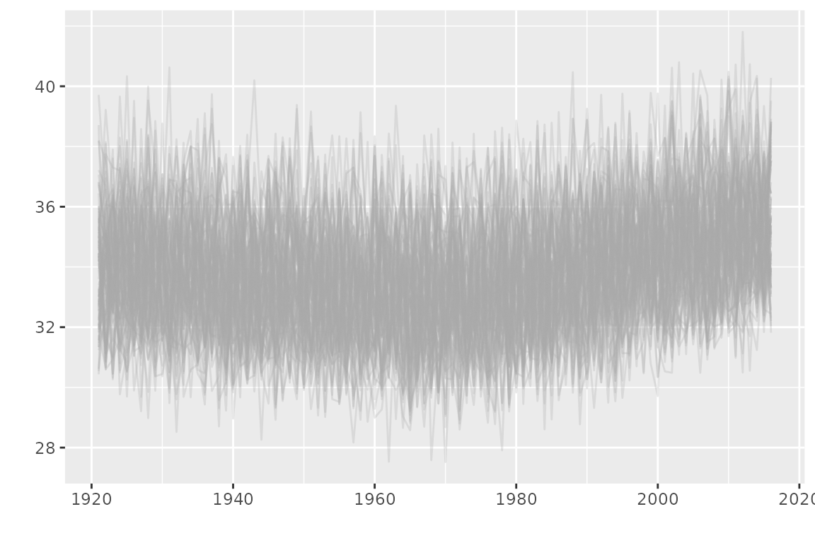
## 6 1926 34.8The data represent the annual maxima of the daily maximal temperature
(TX) in Dijon (France). The time series is shown on the
next plot (R code not shown). The data are provided by European Climate Assessment and
Dataset.
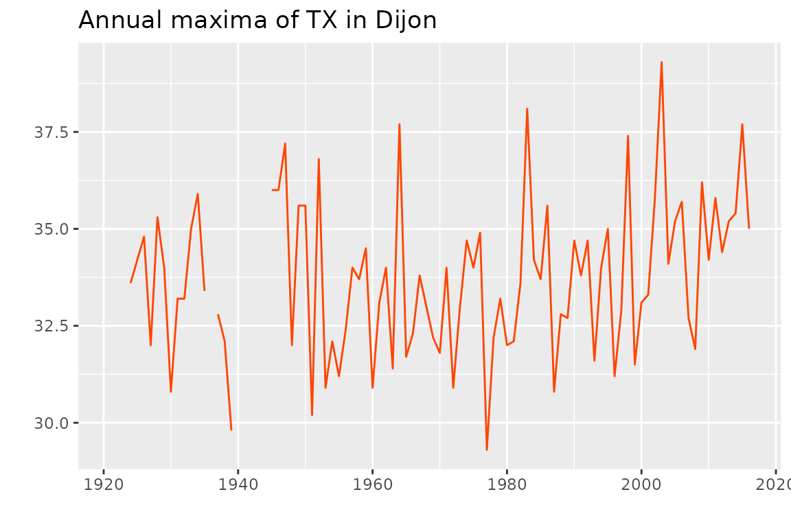
The observations from 1980 on seem to be larger than that of the beginning of the series, motivating the use of a time-varying model.
Simple linear trend
As a possible model, a time-varying block maxima model relates the distribution of the response for the block (year) to the corresponding time , assuming that the observations are independent across blocks. We will assume here that has a GEV distribution with constant scale , a constant shape and a time-varying location . This model involves a vector of four unknown parameters.
We can fit this model by using several CRAN packages, for instance the extRemes package. With this package we need to exclude the missing values for the response
fite1 <- extRemes::fevd(x = TXMax,
                        data = subset(TXMax_Dijon, !is.na(TXMax)),
                        type = "GEV", location.fun = ~Year)
Note that a classical formula is used to specify the model
as it is done for linear models with lm or
glm. By default, a formula implies the use of a constant.
So the formula ~ Year indeed implies the existence of the
coefficient
in
.
We could have used equivalently an explicit constant with
~ 1 + Year. On the contrary, a model with no constant
would have been specified by using the formula ~ Year - 1.
This convention is used by most model fitting functions requiring a
formula in the linear model fashion, and TVGEV will be no
exception.
By inspecting the content of the object or by reading the help, we can find the estimated values of the parameters
fite1$results$par## mu0 mu1 scale shape
## 5.07814887 0.01414038 1.84726804 -0.19990410
fite1$results$value## [1] 180.6135We see that the estimated location increases by about
1.41 Celsius by
century, with an intercept value
5.08 Celsius corresponding to the year
.
We extracted as well the negative maximized log-likelihood stored in the
element results$value.
To achieve nearly the same thing with the NSGEV
package, we need a little extra work: adding a column with class
"Date" to the data frame. Each observation of this date
column represents the beginning of a block. We can simply paste a month
and day indication -mm-dd to the year in order to get a
POSIX format
## [1] "Date"
head(df$Date, n = 5)## [1] "1921-01-01" "1922-01-01" "1923-01-01" "1924-01-01" "1925-01-01"Note that we no longer have to remove the observations with a missing response. Now we can fit the same model
fitNLin <- TVGEV(data = df, response = "TXMax", date = "Date",
               design = polynomX(date = Date, degree = 1),
               loc = ~ t1)
coef(fitNLin)
## mu_0 mu_t1 sigma_0 xi_0
## 32.93752186 0.01527735 1.84567285 -0.20471258
logLik(fitNLin)## [1] -180.6005
## attr(,"df")
## [1] 4
## attr(,"nobs")
## [1] 87Note that we used a formula as before but now the covariate is a
function of the date which is computed by the design function, here
polynomX. The design function essentially returns a numeric
matrix, the column of which can be used as covariates. So the name of
the covariates depend on the design function used. This will be further
explained later.
The estimated parameters are nearly the same as before, except for
the first one - due to a different origin taken for the linear trend.
Indeed, the time origin for R Dates is "1970-01-01". The
maximized log-likelihood is extracted by using the logLik
method which works for many classes of fitted models.
The “fitted model” object has class "TVGEV", and a
number of classical S3 methods with simple interpretation are
implemented
class(fitNLin)## [1] "TVGEV"
methods(class = "TVGEV")## [1] anova autoplot bs cdf cdfMaxFun
## [6] coef confint density influence logLik
## [11] mean modelMatrices moment plot predict
## [16] print profLik psi2theta quantile quantMax
## [21] quantMaxFun residuals simulate summary vcov
## see '?methods' for accessing help and source codeFor example we can use the classical confint method to
display confidence intervals on the parameters
confint(fitNLin)## , , 95%
##
## L U
## mu_0 32.5048 33.3702
## mu_t1 -0.0005 0.0310
## sigma_0 1.5412 2.1502
## xi_0 -0.3489 -0.0605The results (by default based on the delta method) show that is within the interval on the slope , though being very close to the lower bound. The confidence interval on the shape suggest that this parameter is negative.
As is generally the case with the S3 class/methods system for R,
the methods should be used by invoking the generic function,
e.g. confint. However the help for the methods can be found
by using the “dotted” name such as ?confint.TVGEV. A method
implemented for a specific class usually has specific arguments that are
not found in the generic. For instance, the confint method
for the class "TVGEV" has a specific method
argument that allows choosing the inference method, with the three
choices "delta" (default), "boot" and
"proflik".
Stationary model with no trend
Quite obviously, we can fit a model with a constant trend by using the relevant formula
fitNConst <- TVGEV(data = df, response = "TXMax", date = "Date",
                   design = polynomX(date = Date, degree = 1),
                   loc = ~ 1)
coef(fitNConst)
## mu_0 sigma_0 xi_0
## 32.94616 1.87935 -0.19645Since the design function is not used when the three GEV parameters
are constant, we can use TVGEV without its
design argument.
##     mu_0  sigma_0     xi_0
## 32.94616 1.87935 -0.19645Note however that we still require that the response and the date are provided as columns of a data frame.
As a general rule, a time-varying model should always be compared to
a simpler model with three constant GEV parameters. For that aim, we can
perform a likelihood-ratio test, which is by convention attached to the
anova method in R.
anova(fitNConst, fitNLin)## Analysis of Deviance Table
##
## df deviance W Pr(>W)
## fitNConst 3 364.74
## fitNLin 4 361.20 3.5412 0.05986 .
## ---
## Signif. codes: 0 '***' 0.001 '**' 0.01 '*' 0.05 '.' 0.1 ' ' 1The -value is > 0.05, so if we assume that there could be a global linear trend on the location, we would accept the null hypothesis at the level.
We can investigate different forms of trend, using different designs.
Designs and models
Example: polynomial design
Now let us have a look at the design function polynomX
which was used before. We can call it using the date column of the data
frame df passed to the formal argument date of
the function.
## [1] "bts" "matrix"
head(X)## Block time series
##
## o First block: 1921-01-01
## o Last block: 2016-01-01
##
## date Cst t1
## 1921-01-01 1.00000 -48.99932
## 1922-01-01 1.00000 -48.00000
## 1923-01-01 1.00000 -47.00068
## 1924-01-01 1.00000 -46.00137
## 1925-01-01 1.00000 -44.99932
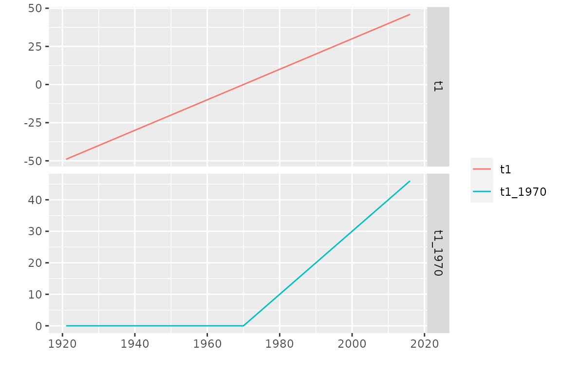
## 1926-01-01 1.00000 -44.00000The result is an object with class "bts", inheriting
from the class "matrix", with two columns. We guess that
the column named Cst is a column of ones as commonly used
in linear regression, and that the column t1 is a linear
trend in years with its origin set 49 years after 1921-01-01, so near
1970-01-01. Note that a TVGEV model does not need to use
all the basis functions of the design: we did not use the constant
Cst, because a constant basis function is generated by
default when the formula is parsed.
The class "bts" describes objects representing block
times series. It is quite similar to the "mts" class of the
forecast package. A few methods are implemented for
this class e.g. the autoplot method. To illustrate this
method, we consider a different design function involving broken line
splines, namely the function breaksX
The basis functions are now splines with degree
.
The first function named t1 is a linear function and for
each “break” date given in breaks, a broken line function
is added to the basis.
There are other design functions. These are consistently used in
TVGEV as follows.
Using designs with TVGEV
With TVGEV
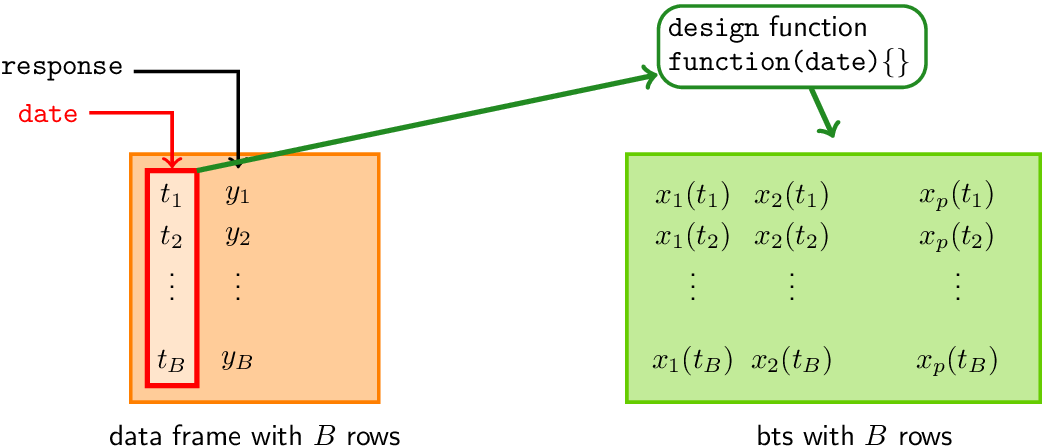
When the model is fitted, the data frame specified with the
dataformal argument must contain a column giving the date of the beginning of each block. The column name is specified by using thedateformal argument ofTVGEV.The date column is passed to a design function given in the
designformal argument. The value ofdesignis a call to the chosen function, using the chosen column ofdataas thedateof the design function.The block maxima model is specified through formulas linking the GEV parameters to the columns of the design matrix.
The fitted model object keeps track of the design function used and therefore can use it on a “new” period of time to make a prediction.
Broken line trend on the location
We can use the breaksX design function to specify a
continuous broken line form for the location
.
fitNBreak <- TVGEV(data = df, response = "TXMax", date = "Date",
               design = breaksX(date = Date, breaks = "1970-01-01", degree = 1),
               loc = ~ t1 + t1_1970)
coef(fitNBreak)
## mu_0 mu_t1 mu_t1_1970 sigma_0 xi_0
## 32.06638460 -0.02392656 0.07728411 1.75541862 -0.18112018The location parameter now involves three parameters according to
where
is the “positive part” function and where
corresponds to the break point in time. Note that the slope of the
location
is given by
before the break point, and by
after that point. This corresponds to the two estimated slopes in
Celsius by century:
-2.4 (before break) and
5.3 (after). Since
represents the change of slope, we could decide whether the change of
slope is significant or not by querying whether a confidence interval on
contains
or not. Another solution based on anova is described
later.
To assess the change in the distribution of
,
many graphical diagnostics can be produced with NSGEV.
For instance we can use the quantile method, which produces
a bts block time-series that can be autoplotted
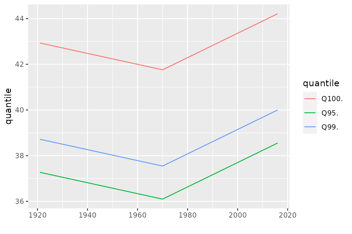
Since the estimated value of the shape parameter is negative, all the GEV distributions for the observations are estimated as having a finite upper end-point . We can find this value by setting the probability to in the quantile function. Remind that we use the estimated distribution, so the shown upper end-point is the estimate . We could infer on the unknown value by using confidence intervals. The value of is the return level (conditional on ) corresponding to an infinite return period .
The two models corresponding to the objects fitNLin and
fitNBreak are nested: by setting
in the second model, we retrieve the first one. So we can perform a
likelihood-ratio test as above.
anova(fitNLin, fitNBreak)## Analysis of Deviance Table
##
## df deviance W Pr(>W)
## fitNLin 4 361.2
## fitNBreak 5 354.4 6.7982 0.009125 **
## ---
## Signif. codes: 0 '***' 0.001 '**' 0.01 '*' 0.05 '.' 0.1 ' ' 1We see from the very small
-value
labelled Pr(>W) that the null hypothesis
must be rejected in favour of a break at the chosen break time as
defended by fitNBreak.
A limitation of the fitNBreak model is that the break
time can not be estimated simply. The same problem arises for the
Gaussian regression known as kink regression. So we can try
another basis of slowly varying functions which is flexible enough to
describe a smooth transition between two linear trends with different
slopes.
Natural spline basis
As a third example of design, we will use the natural spline
design as implemented by natSplineX. With this design, we
need to give two boundary knots as well as a number of knots between the
boundary knots. Along with its flexibility, an interesting property of
this basis is that the extrapolation outside of the boundary knots is
“only” linear. By using polynomials of degree
,
we would get a quadratic trend which becomes unrealistic even for a
small amount of extrapolation.
X1 <- natSplineX(date = df$Date, knots = "1970-01-01",
                 boundaryKnots = c("1921-01-01", "2017-01-01"))
autoplot(X1, facets = TRUE)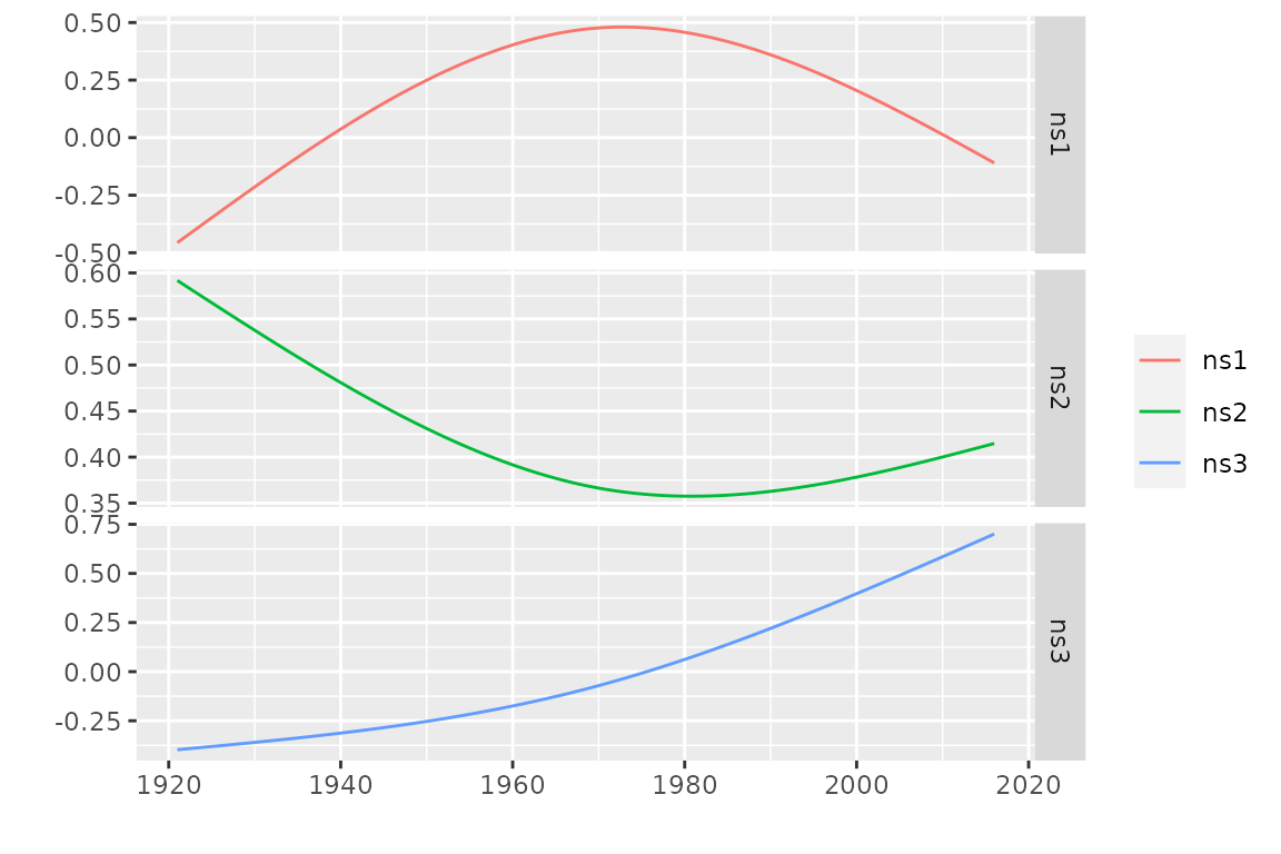
The basis functions are linearly independent but they span a linear
space which contains the constant
;
in other words, if we add a column of ones to unclass(X1)
we get a matrix with four columns but with rank
.
So we can either use a constant and two of the basis functions, or use
the three basis function but we then have to remove the default
constant as follows.
fitNNS <- TVGEV(data = df, response = "TXMax", date = "Date",
               design = natSplineX(date = Date, knots = "1970-01-01",
                   boundaryKnots = c("1920-01-01", "2017-01-01")),
               loc = ~ ns1 + ns2 + ns3 - 1)
As before the models corresponding to fitNLin and
fitNNS are nested because the basis functions used in
fitNLin (the implicit constant
and the linear function t1) both are in the linear space
generated by the natural spline basis. So we can use the
anova method.
anova(fitNLin, fitNNS)## Analysis of Deviance Table
##
## df deviance W Pr(>W)
## fitNLin 4 361.20
## fitNNS 5 354.14 7.0651 0.00786 **
## ---
## Signif. codes: 0 '***' 0.001 '**' 0.01 '*' 0.05 '.' 0.1 ' ' 1Again we see that fitNNS fits the data significantly
better than fitNLin does. We can not compare the two models
fitNBreak and fitNNS by using
anova because they are no longer nested. However since
these two models have the same number of parameters, using AIC or BIC
would conclude to a slight advantage in favour of fitNNS
which has a slightly smaller deviance, hence a slightly larger
log-likelihood.
##         Breaks Natural Spline
##       376.7323       376.4654
Possible numerical problems
A possible source of problems, the design matrices created by the
design functions can take large values. Indeed, a date is considered as
a number of days for a given origin; for a long series we will get basis
functions with values of several thousands or even much more when
polynomials with degree
are used. In order to facilitate the task of maximizing the likelihood,
it is worth using the origin formal argument of the
provided design functions, setting it to a date close to the mean date
of the series.
Return levels and quantiles
Conditional return levels
With time-varying models or non-stationary models, the concept of return level becomes quite messy, because many reasonable definitions can be given. The simplest return levels are the conditional ones, obtained by fixing a time and by considering the quantiles of the fitted distribution for that specific time.
pBreak <- predict(fitNBreak)## Since 'object' is really time-varying, the Return Levels
## depend on the date. A default choice of dates is made here.
## Use the 'newdate' formal to change this.
autoplot(pBreak)## Warning: Using `size` aesthetic for lines was deprecated in ggplot2 3.4.0.
## ℹ Please use `linewidth` instead.
## ℹ The deprecated feature was likely used in the NSGEV package.
## Please report the issue at <https://github.com/IRSN/NSGEV/issues/>.
## This warning is displayed once per session.
## Call `lifecycle::last_lifecycle_warnings()` to see where this warning was
## generated.## ~Date
## <environment: 0x562454958348>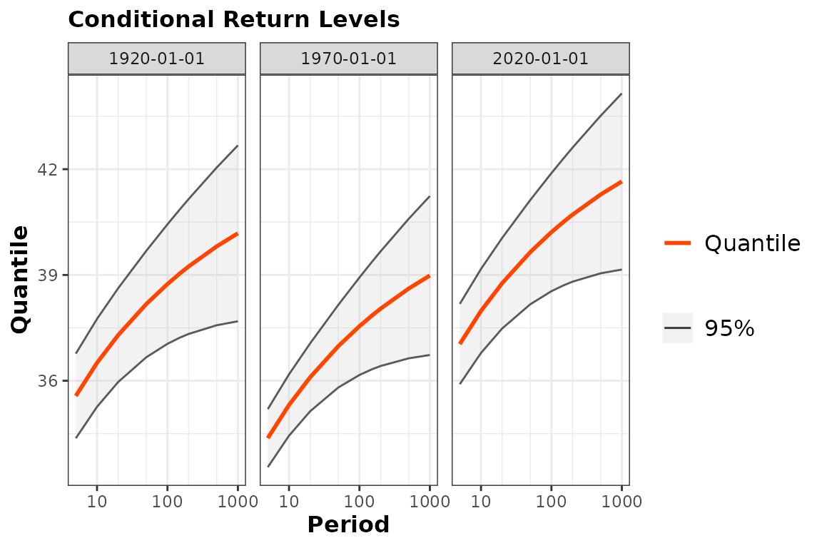
As suggested by the warning message, three “round” values are chosen
by default for the time
and the return level plots are shown for each of these in a specific
facet of the plot. Note that the axis could have used a probability of
exceedance on a yearly basis rather than a period in years. We can make
a different choice by using the newdate optional argument
of predict, see ?predict.TVGEV.
Confidence Intervals
Each of the return levels is computed with a confidence interval with
its default level set to
.
By default, the delta method is used, resulting in symmetrical
confidence intervals. Two alternative methods can be used by setting the
optional argument confintMethod: profile-likelihood and
bootstrap. With the profile-likelihood method, a constrained
optimization method is repeatedly used and convergence diagnostics are
printed by default. To save space we remove these by setting the
trace argument.
pBreakPL <- predict(fitNBreak, confintMethod = "proflik", trace = 0)## Since 'object' is really time-varying, the Return Levels
## depend on the date. A default choice of dates is made here.
## Use the 'newdate' formal to change this.
plot(pBreakPL)## Warning in plot.predict.TVGEV(pBreakPL): Inasmuch the plot is actually a
## 'ggplot', it is better to use the 'autoplot' method for consistency## ~Date
## <environment: 0x5624503002b0>Unconditional return levels
Unconditional return levels can be defined for the time-varying framework. These are obtained by aggregating several times corresponding to a prediction period. Many definitions are possible; a natural requirement is that the usual definition continues to hold when a stationary model is considered as time-varying.
Following Parey et al (Parey, Sylvie and Hoang, Thi Thu Huong and Dacunha-Castelle, Didier 2010), we can define the return level corresponding to years as the level such that the number of exceedances over in the “next years” has unit expectation . The notion of “next” year is relative to a time origin that can be chosen.
pUCBreak <- predictUncond(fitNBreak, newdateFrom = "2020-01-01",
                          confintMethod = "proflik", trace = 0)
plot(pUCBreak)
## Warning in plot.predict.TVGEV(pUCBreak): Inasmuch the plot is actually a
## 'ggplot', it is better to use the 'autoplot' method for consistency
kable(pUCBreak, digits = 2)| Date | Period | Level | Quant | L | U |
|---|---|---|---|---|---|
| 2020-01-01 | 5 | 95% | 37.15 | 35.97 | 38.38 |
| 2020-01-01 | 10 | 95% | 38.23 | 36.95 | 39.62 |
| 2020-01-01 | 20 | 95% | 39.31 | 37.82 | 41.00 |
| 2020-01-01 | 30 | 95% | 40.04 | 38.33 | 42.01 |
| 2020-01-01 | 40 | 95% | 40.65 | 38.71 | 42.89 |
| 2020-01-01 | 50 | 95% | 41.22 | 39.03 | 43.72 |
| 2020-01-01 | 70 | 95% | 42.30 | 39.57 | 45.36 |
| 2020-01-01 | 100 | 95% | 43.90 | 40.29 | 47.85 |
For instance the return level corresponding to
years for the origin "2020-01-01" should be exceeded once
(on average) during the 30 years 2021 to 2050. This level is estimated
here to be 40.04 Celsius.
Note that an alternative definition of the return level can be
implemented as a function
of the parameter vector
of the model. Under quite general conditions, such a return level can be
regarded as a parameter of the model in a re-parameterization of it,
hence we can infer on it as we do for a parameter. To achieve this in
practice, the return level must be implemented as a R function with
signature function(object, psi) where object
has class "TVGEV" and psi stands for the
parameter vector. The profLik method can then be used to
infer on the return level using the profile-likelihood method, see
?profLik.TVGEV. This method can work for any smooth
function having the previous signature.
Quantiles of the maximum
Rather than trying to generalize the definition of a return level to the time-varying framework, one can simply consider the random maximum where the maximum is over a set of blocks. The most common case is when is a future period , , , such as the lifetime or design life (Rootzén and Katz 2013) of an equipment, and one want to assess a risk related to the possible exceedance over some high level during this period. Since the blocks are assumed to be independent we have
where the dependence on the parameter is through . Note that in general does not follow a GEV distribution.
The corresponding quantile function can be computed numerically either by solving or by interpolating from couples of values probability, quantile . For a given probability , the derivative of the corresponding quantile w.r.t. can be obtained by the implicit function theorem and can be used to infer on the quantile.
In NSGEV, the quantMax method can be
used to produce a table of values for the quantile function from a
TVGEV object. Such a table is given the S3 class
"quantMax.TVGEV" for which an autoplot method
has been implemented
newDate <- as.Date(sprintf("%4d-01-01", 2025:2054))
qM <- quantMax(fitNBreak, date = newDate, level = c(0.70, 0.95))
gqM <- autoplot(qM) +
    ggtitle("Maximum on years 2025-2054 with delta confidence intervals")
print(gqM)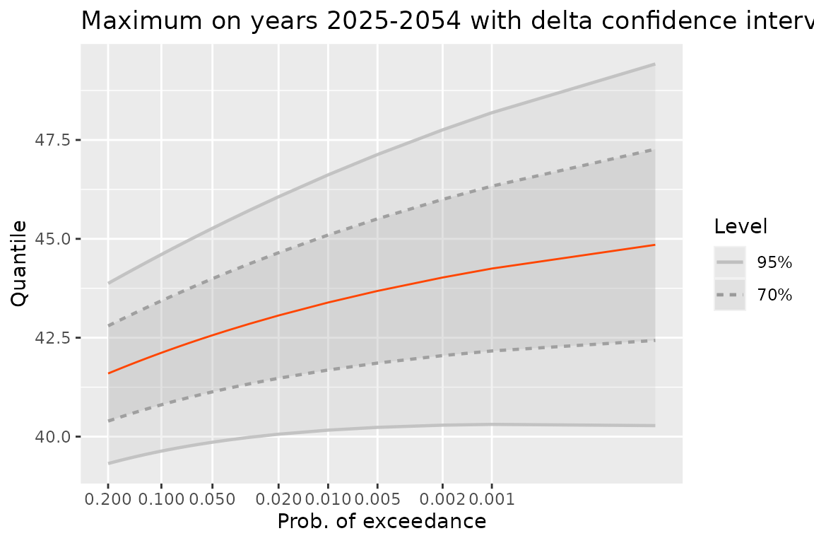
The plot shows the quantile against the probability of exceedance using a Gumbel scale. So if happens to be Gumbel (as can happen in the stationary case) the quantile line will be a straight line. When the period of interest is increased the maximum becomes stochastically larger. For instance, with a fixed beginning if the duration of the period is increased the maximum becomes stochastically larger: all quantiles are increased.
It is worth noting that as far as a small probability of exceedance is concerned, the expected value of the random number of exceedances over the corresponding quantile is . This approximation is acceptable when .
On the previous plot, confidence intervals based on the delta method are shown. It is now possible to use profile likelihood intervals, at the price of an increased computation time.
qM2 <- quantMax(fitNBreak, date = newDate, level = c(0.70, 0.95),
                confint = "proflik")
gqM2 <- autoplot(qM2) +
    ggtitle("Maximum on years 2025-2054 with profile likelihood  intervals")
print(gqM2)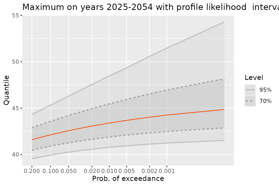
Needless to say, for a small probability of exceedance, the upper bound of the profile likelihood confidence interval is much larger than that of the delta interval.
Simulate from a fitted model
The simulate method is implemented in many R packages,
with the aim to simulate new data from a given model. It has been
implemented for the TVGEV class. A fitted model object can
be used to simulate new paths either for the fitting time period or for
a new one.
We can use a different period to better understand how the model anticipates new data
nd <- seq(from = as.Date("2020-01-01"), length = 10, by = "years")
autoplot(simulate(fitNBreak, nsim = 10, newdate = nd))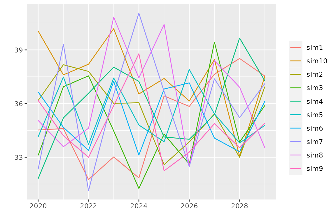
The simulated paths are here drawn in colour with a legend because
their number is small enough. Note that simulate is
functionally close to a prediction: the mean of a large number of
simulated paths is close to the expectation used in a prediction and the
uncertainty on the prediction can be assessed by using the dispersion of
the simulated paths.
More diagnostics and results
Residuals
The generalized residuals are random variables
related to the observations
,
so they form a block time-series. The distribution of
should be nearly the same for all blocks
and the dependence between the blocks should be weak (Cox and Snell 2018). Several definitions of the
residuals are possible, in relation with a target distribution. A simple
choice is
which should lead nearly to a uniform distribution on the interval
.
Other possible choices are
for a standard exponential target as used by Panagoulia, Economou, and Caroni (2014) and by
Katz, Parlange, and Naveau (2002), or
for a standard Gumbel target. Note that the resid method of
the package uses an increasing transformation so that
large/small residuals correspond to large/small observations. When the
GEV marginal distributions have a nearly exponential tail
using the standard Gumbel target for the generalized residuals can be
preferred because this will use a milder transformation of the data.
This is now the default choice.
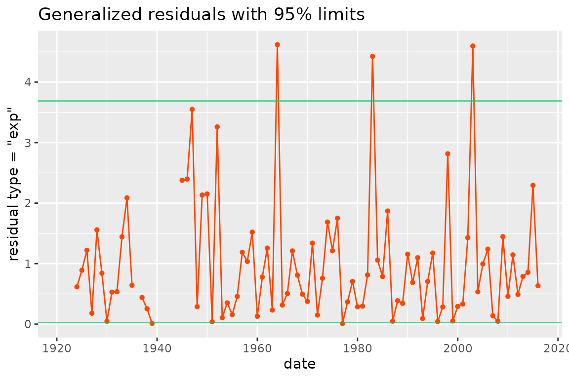
The horizontal lines show an interval with approximate probability . The use of these residuals is similar to that in the usual linear regression framework where the distribution of the standardized residuals is close to the standard normal.
Parameters: “psi” vs “theta”
As shown before the parameters of the model can be extracted by using
the coef method. Using a non-standard terminology which
seems specific to the package, we can say that these are the “psi”
parameters. But we can be interested as well by the GEV parameters
,
and
that we can call “theta”
.
Since these parameters depend on the time
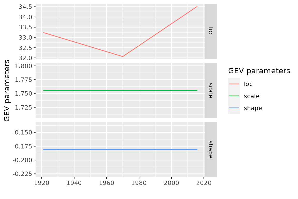
we can consider them as forming a block time series. We can “extract”
these parameters by using the optional formal type of the
coef method; this leads to a bts object that
can be autoplotted. Remind that the physical dimensions of the
parameters differ -
and
have the dimension of the
while
is dimensionless - so we have better show each series in a facet with
its own
axis.
Marginal distributions
Several methods can be used to assess the marginal distribution of
for a specific time
or at a collection of times given by a date argument. With
the default date = NULL, the methods quantile,
mean, moments for the class
"TVGEV" return time series objects that can be
“autoplotted” to plot the quantiles or the mean (expectation) against
the date as it was shown before. The help page with examples can be
displayed in the usual way, e.g. with ?quantile.TVGEV.
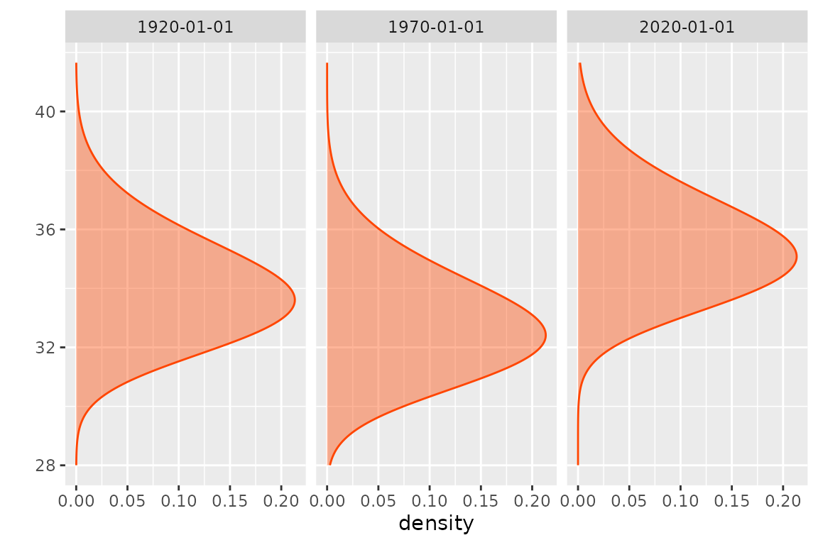
The density and cdf methods both return a
functional time series: a collection of functions depending on the date.
These can be autoplotted as well.
If needed, the time series with class "bts" can be
coerced into a standard time series inheriting from "ts"
for which many methods have been written in different packages.
Bootstrap
Principle
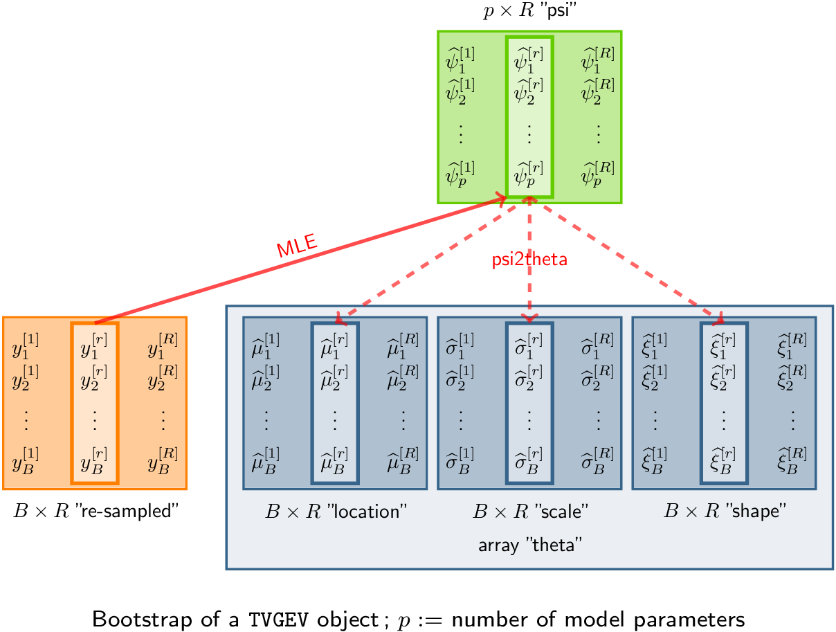
A large number of response vectors are simulated or “re-sampled” corresponding to , , . These simulated values can be stored into a matrix with rows and columns. For each vector , the MLE of the “psi” parameter vector is computed. The sample quantiles of the can then be used to provide a confidence interval on .
The bs method takes a TVGEV object as its
first argument and computes the bootstrapped “psi” parameters
.
These bootstrapped parameters are in fact stored as the rows of the
estimate element of the returned list.
myBoot <- bs(fitNBreak) ## The optimisation failed to converge. Hints: give `psi0`, try using `estim = "nloptr", give lower and upper bounds.## Warning in MLE.TVGEV(object, y = y[, b], estim = estim, ...): convergence not
## reached in optimisation
names(myBoot)## [1] "estimate" "negLogLik" "R" "optim" "type"
head(myBoot$estimate, n = 3)## mu_0 mu_t1 mu_t1_1970 sigma_0 xi_0
## [1,] 32.18540 -0.02209687 0.07976180 1.901520 -0.2294907
## [2,] 31.72127 -0.04716687 0.09096013 1.613856 -0.1025511
## [3,] 31.90407 -0.02768300 0.08830328 1.636649 -0.1734725Note that the default number of replicates R is very
small and has been set for a purely illustrative use. A well-accepted
choice
.
It is easy to derive from the theta parameters the corresponding
block times series of “thetas”
.
Broadly speaking we have to apply the function psi2theta to
each line of the matrix returned as the estimate element of
the result.
mu <- apply(myBoot$estimate, MARGIN = 1,
            FUN = function(x, model) psi2theta(psi = x, model = model)[ , 1],
            model = fitNBreak)
autoplot(bts(mu, date = fitNBreak$fDate)) + ggtitle("bootstrapped values for mu")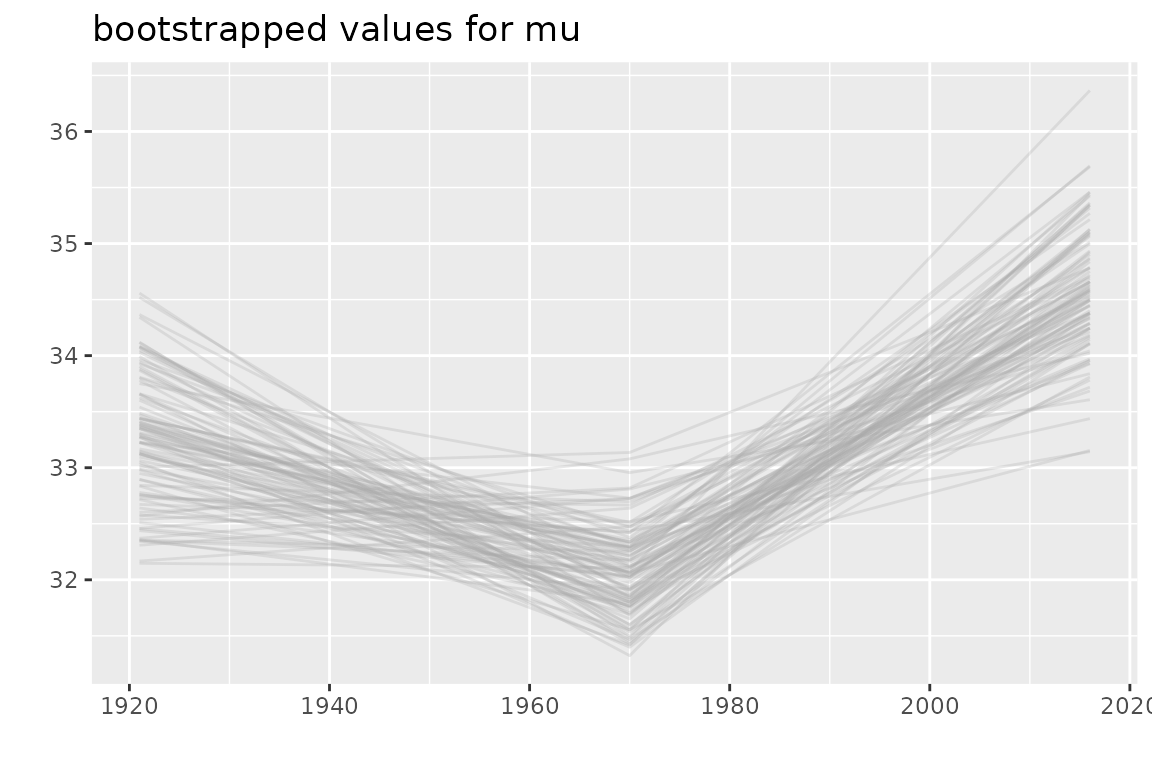
One the bootstrapped values for the “psi” parameters have been
computed, they can be used to later infer on the return periods at a
short computing cost. In that aim, a new element named boot
must be added to the fitted model.
fitNBreak$boot <- myBootNote however that this is a kind of “hack”. Some care is needed to
ensure that the new boot element is consistent with the
right fitted model using the right data.
Since most modern computers use multicore processors, a parallel
computation can be used to achieve substantial saving in the computing
time. See the example in the help page of boot.ts to see
how this can be achieved.
Details how resampling is performed
Two methods can be used to “resample” (Panagoulia, Economou, and Caroni 2014)
Parametric. For , , , the value is drawn as where is the MLE of the vector of the three GEV parameters corresponding to the block , which is a function of .
Non-parametric. For , , , the generalized residuals are resampled to form a vector with the wanted size . Each residual is back-transformed to a response .
The second method is also known under the names fixed- resampling and resampling from the residuals.
The bootstrap can also be used to infer on the return levels, either conditional or unconditional. For example, the conditional return level corresponding the the period of blocks and for the given time can be inferred by using the quantiles of the return periods which are computed as for .
Strengths and limitations of TVGEV
The "TVGEV" S3 class and its dedicated methods allow a
simple use of time-varying GEV models, including prediction. Some
functionality of the package such as the simulation are not found in
more classical packages, to our best knowledge. However
Only known functions of time can be used as covariates.
Each of GEV parameters can only depend on the time covariates through a linear function of these.
The parameters can not be share across GEV parameters.
To illustrate 1., we can not use a binary variable indicator of a site in order to build a regional model. To illustrate 2., the GEV location can be but not have the form . To illustrate 3., we can not have both and , because the parameters and are then used both by the location and the scale .
Appendix
Coping with dates
In practice, the time will be represented by a date object,
and the POSIX format "yyyy-mm-dd" or in R
"%Y-%m-%d" will be favored. The R base
package has a "Date" class which is used by
NSGEV
## [1] "Date"
myDate## [1] "2020-01-01"
format(myDate, "%d %B %Y")## [1] "01 January 2020"
myDate <- seq(from = as.Date("1980-01-01"), by = "years", length = 40)
x <- runif(length(myDate))
plot(myDate, x, type = "o", xlab = "")
The lubridate package (Grolemund and Wickham 2011) has functions that can help to cope with date.
Adding new design functions
You can add new design functions. A design function:
Must have its first argument named
date. This argument is intended to be passed either as an object with class"Date"or as an object which will be coerced automatically to this class by usingas.Date. For instance, a character vector in POSIX format should work.Must return a matrix with the basis function as its columns. It must also have an attribute named
"date"containing the date vector. This object should be created either by using thebtsfunction (creator for the class) or by simply giving the classc("bts", "matrix")to a matrix with the suitable attribute.
Estimating the break with a broken line trend
Let us consider again the broken line trend discussed above, namely
As mentioned before, the date
of a change of slope can be considered as an unknown parameter, but the
model then no longer has the form for TVGEV objects, so it
can no longer be estimated by using directly the TVGEV
function. Yet we can find the value of
by maximizing the log-likelihood over a vector of candidate values:
estimating a TVGEV model for each value will provide the
corresponding log-likelihoods. For a given year we can create a suitable
formatted date with the sprintf function as follows
yearBreaks <- c(1940, 1950, 1955, 1960:2000, 2005, 2010)
res <- list()

for (ib in seq_along(yearBreaks)) {
    d <- sprintf("%4d-01-01", yearBreaks[[ib]])
    floc <- as.formula(sprintf("~ t1 + t1_%4d", yearBreaks[[ib]]))
    res[[d]] <- TVGEV(data = df, response = "TXMax", date = "Date",
                      design = breaksX(date = Date, breaks = d, degree = 1),
                      loc = floc)
}
## Warning in TVGEV(data = df, response = "TXMax", date = "Date", design = breaksX(date = Date, : 'design' uses variables not in `data`: `d`.
## This may be a source of problems in scoping, because these variables are
## at the best found in an environment differing from `data`. See the vignette `Using variables in the design argument of TVGEV`.
## Warning in TVGEV(data = df, response = "TXMax", date = "Date", design = breaksX(date = Date, : 'design' uses variables not in `data`: `d`.
## This may be a source of problems in scoping, because these variables are
## at the best found in an environment differing from `data`. See the vignette `Using variables in the design argument of TVGEV`.We now have a list res of
length(yearBreaks) objects and the log-likelihood of each
object can be extracted by using logLik. So we can plot the
log-likelihood against the year and find the “best” object with maximal
log-likelihood.
ll <- sapply(res, logLik)
plot(yearBreaks, ll, type = "o", pch = 21, col = "orangered",
     lwd = 2, bg = "gold", xlab = "break", ylab = "log-lik")
grid()
iMax <- which.max(ll)
abline(v = yearBreaks[iMax])
abline(h = ll[iMax] - c(0, qchisq(0.95, df = 1) /2),
       col = "SpringGreen3", lwd = 2)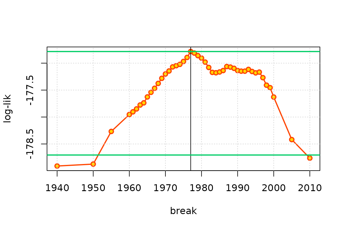
Although the points show a profiled log-likelihood, the regularity conditions that must hold in ML estimation are not fulfilled, because the log-likelihood is not differentiable w.r.t. . As a consequence, the usual level (shown as the lower horizontal line in green here) does not provide a confidence interval on the unknown .
Constraints on the parameters, fixed parameters
As an experimental feature, inequality constraints on the parameters
can be imposed. The constraints are simple “box” constraints of the form
where
and
are given. These constraints can only be used when the likelihood is
maximized with the nloptr package. If needed, they can be
given for some parameters only, letting the other bounds fixed at their
default values
and
.
In practice, the constraints are given by using a named vector, and
hence the names of the parameters must be known. These names can be
retrieved if needed by first using estim = "none".
fitNBreak2 <-
    TVGEV(data = df, response = "TXMax", date = "Date",
          design = breaksX(date = Date, breaks = "1970-01-01", degree = 1),
          loc = ~ t1 + t1_1970,
          estim = "nloptr",
          coefLower = c("xi_0" = -0.15), coefUpper = c("xi_0" = 0.0))
## Warning in MLE.TVGEV(object = tv, y = NULL, psi0 = psi0, estim = estim, : some
## estimated parameters at the bounds, inference results are misleading
coef(fitNBreak2)## mu_0 mu_t1 mu_t1_1970 sigma_0 xi_0
## 32.02318423 -0.02420594 0.07812270 1.72977928 -0.15000000The GEV shape parameter is usually taken as constant, not time-varying; inasmuch the log-likelihood is when , a lower bound should normally be set. In practice, this is usually not needed because for numerical reasons the optimization will converge to a local maximum with and a finite log-likelihood rather than to a parameter vector with the infinite maximal log-likelihood.
The constraints can be used to set a parameter to a given value by taking and .
fitNBreak3 <-
    TVGEV(data = df, response = "TXMax", date = "Date",
          design = breaksX(date = Date, breaks = "1970-01-01", degree = 1),
          loc = ~ t1 + t1_1970,
          estim = "nloptr",
          coefLower = c("mu_t1" = -0.02, "xi_0" = -0.2),
          coefUpper = c("mu_t1" = -0.02, "xi_0" = 0.1))
## Warning in MLE.TVGEV(object = tv, y = NULL, psi0 = psi0, estim = estim, : some
## estimated parameters at the bounds, inference results are misleading
coef(fitNBreak3)## mu_0 mu_t1 mu_t1_1970 sigma_0 xi_0
## 32.13623265 -0.02000000 0.07108756 1.75700613 -0.18234029