Goal
In this report, we compare profile-likelihood inference results given by NSGEV with those of other packages, mainly ismev. We make use of classical data.
Port Pirie data
ML Estimation
library(ismev)
data(portpirie, package = "ismev")
df <- portpirie
df <- within(df, date <- as.Date(sprintf("%4d-01-01", Year)))
fitNSGEV <- try(TVGEV(data = df, response = "SeaLevel", date = "date"))
fitismev <- gev.fit(xdat = df$SeaLev)
## $conv
## [1] 0
##
## $nllh
## [1] -4.339058
##
## $mle
## [1] 3.87474692 0.19804120 -0.05008773
##
## $se
## [1] 0.02793211 0.02024610 0.09825633
fitextRemes <- extRemes::fevd(x = df$SeaLev, type = "GEV")

rbind("NVSGEV" = coef(fitNSGEV),
      "ismev" = fitismev$mle,
      "extRemes" = fitextRemes$results$par)
## mu_0 sigma_0 xi_0
## NVSGEV 3.874751 0.1980449 -0.05012018
## ismev 3.874747 0.1980412 -0.05008773
## extRemes 3.874750 0.1980440 -0.05010950Confidence Intervals on Parameters
The check_confint function checks the computation of the
profile-likelihood intervals on the shape parameter. This is a graphical
test: on the plot produced by ismev::prof.xi, we add two
green vertical lines showing the confidence limits for the shape
parameter given by the confint method for the class
"TVGEV". We must check that both lines cut the
profile-likelihood curve at a point with an ordinate matching the lowest
horizontal blue line.
check_confint(fitNSGEV, ref = fitismev, level = 0.95)##
##
## o Finding CI for "mu_0"
##
## o 95%, lower bound: 3.82
## Constraint check 0.0000000, -2.4183
## 95%, upper bound: 3.93
## Constraint & value -0.0000030, -2.4183
##
##
## o Finding CI for "sigma_0"
##
## o 95%, lower bound: 0.16
## Constraint check -0.0000000, -2.4183
## 95%, upper bound: 0.24
## Constraint & value -0.0000000, -2.4183
##
##
## o Finding CI for "xi_0"
##
## o 95%, lower bound: -0.22
## Constraint check -0.0000000, -2.4183
## 95%, upper bound: 0.17
## Constraint & value -0.0000000, -2.4183
## If routine fails, try changing plotting interval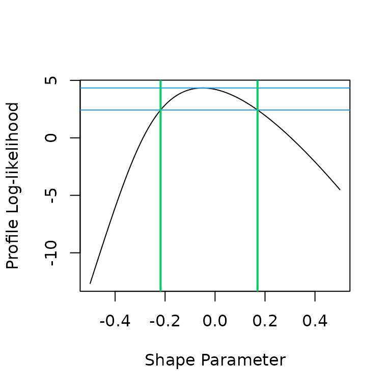
Confidence level 95%.
check_confint(fitNSGEV, ref = fitismev, level = 0.70)##
##
## o Finding CI for "mu_0"
##
## o 70%, lower bound: 3.85
## Constraint check -0.0000000, -3.8020
## 70%, upper bound: 3.90
## Constraint & value -0.0000000, -3.8020
##
##
## o Finding CI for "sigma_0"
##
## o 70%, lower bound: 0.18
## Constraint check -0.0000000, -3.8020
## 70%, upper bound: 0.22
## Constraint & value -0.0000001, -3.8020
##
##
## o Finding CI for "xi_0"
##
## o 70%, lower bound: -0.14
## Constraint check -0.0000001, -3.8020
## 70%, upper bound: 0.06
## Constraint & value 0.0000000, -3.8020
## If routine fails, try changing plotting interval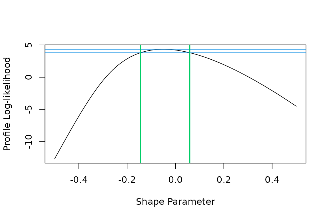
Confidence level 70%.
Confidence Intervals on Return levels
The check_predict function checks the computation of the
profile-likelihood confidence intervals on return levels. As for
check_confint, the check is essentially graphical. On each
plot, the two vertical lines show the confidence limits given by the
predict method for the class "TVGEV". We must
check that both lines cut the profile-likelihood curve at a point with
an ordinate matching the lowest horizontal blue line.
check_predict(fitNSGEV, ref = fitismev, level = 0.95)
Confidence level 95%.
check_predict(fitNSGEV, ref = fitismev, level = 0.70)
Confidence level 70%.
Note that the function is rather verbose, so the results have been hidden.
Fremantle data
ML Estimation
library(ismev)
data(fremantle, package = "ismev")
df <- fremantle
df <- within(df, date <- as.Date(sprintf("%4d-01-01", Year)))
fitNSGEV <- try(TVGEV(data = df, response = "SeaLevel", date = "date"))
fitismev <- gev.fit(xdat = df$SeaLev)
## $conv
## [1] 0
##
## $nllh
## [1] -43.56663
##
## $mle
## [1] 1.4823409 0.1412671 -0.2174320
##
## $se
## [1] 0.01672502 0.01149461 0.06377394
fitextRemes <- extRemes::fevd(x = df$SeaLev, type = "GEV")

rbind("NVSGEV" = coef(fitNSGEV),
      "ismev" = fitismev$mle,
      "extRemes" = fitextRemes$results$par)
## mu_0 sigma_0 xi_0
## NVSGEV 1.482298 0.1412784 -0.2172317
## ismev 1.482341 0.1412671 -0.2174320
## extRemes 1.482342 0.1412723 -0.2174282Confidence Intervals on Parameters
check_confint(fitNSGEV, ref = fitismev, level = 0.95)##
##
## o Finding CI for "mu_0"
##
## o 95%, lower bound: 1.45
## Constraint check -0.0000000, -41.6459
## 95%, upper bound: 1.52
## Constraint & value -0.0000001, -41.6459
##
##
## o Finding CI for "sigma_0"
##
## o 95%, lower bound: 0.12
## Constraint check -0.0000000, -41.6459
## 95%, upper bound: 0.17
## Constraint & value -0.0000000, -41.6459
##
##
## o Finding CI for "xi_0"
##
## o 95%, lower bound: -0.33
## Constraint check -0.0000000, -41.6459
## 95%, upper bound: -0.08
## Constraint & value -0.0000000, -41.6459
## If routine fails, try changing plotting interval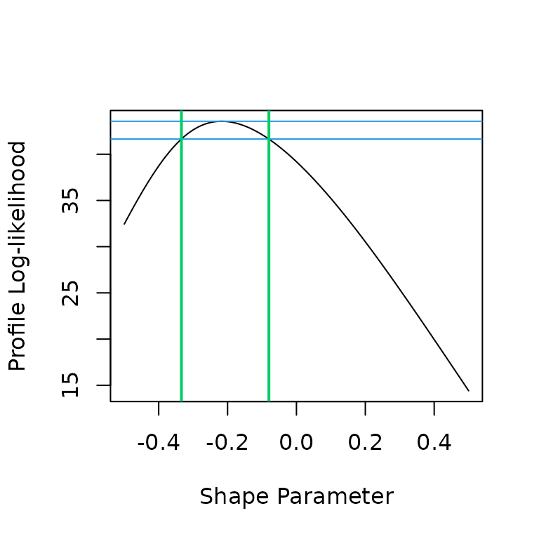
Confidence level 95%.
check_confint(fitNSGEV, ref = fitismev, level = 0.70)##
##
## o Finding CI for "mu_0"
##
## o 70%, lower bound: 1.46
## Constraint check 0.0000000, -43.0295
## 70%, upper bound: 1.50
## Constraint & value -0.0000000, -43.0295
##
##
## o Finding CI for "sigma_0"
##
## o 70%, lower bound: 0.13
## Constraint check -0.0000000, -43.0295
## 70%, upper bound: 0.15
## Constraint & value -0.0000001, -43.0295
##
##
## o Finding CI for "xi_0"
##
## o 70%, lower bound: -0.28
## Constraint check -0.0000000, -43.0295
## 70%, upper bound: -0.15
## Constraint & value -0.0000000, -43.0295
## If routine fails, try changing plotting interval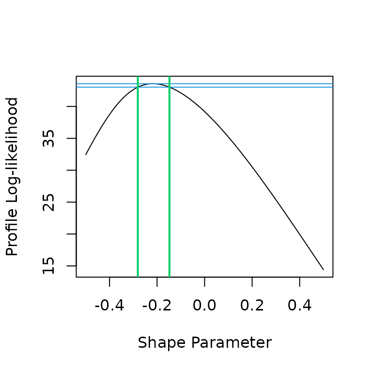
Confidence level 70%.
Confidence Intervals on Return levels
check_predict(fitNSGEV, ref = fitismev, level = 0.95)
Condidence level 95%.
check_predict(fitNSGEV, ref = fitismev, level = 0.70)
Confidence level 70%.