Timeseries Covariates with NSGEV

Yves Deville

2026-01-01

Using timeseries covariates in TVGEV models

In Time-Varying GEV models, a series $y(t)$ of block maxima is considered as formed by independent GEV observations with their marginal distribution depending on the time $t$. In some cases one may want to further use one or several timeseries covariate $z(t)$. A typical example of such timeseries covariates is provided by so-called climate indices such as the Southern Oscillation Index (SOI) and the North Atlantic Oscillation (NAO) both available from the USA National Oceanic and Atmospheric Administration. The response $y(t)$ usually being a timeseries of annual maxima, each covariate $z(t)$ must also come with a yearly sampling, which may require some kind of aggregation using the annual mean or maximum. Most often, timeseries covariates should be used along with functions of time describing the trend, in order to avoid spurious regression, see below. Note that a covariate $z(t)$ does not need to have independent observations nor even to be stationary. The crucial assumption in the model is that the observations $y(t)$ are independent conditional on the series $z(t)$.

Example: Annual Sea Levels in Fremantle (AUS)

The fremantle data of the ismev package contains the annual maxima of the sea level in Fremantle, Australia, in meters. This dataset is described in Chap. 1 of Coles (2001) and is used in Chap. 6 of the book to provide examples of models for non-stationary extremes.

library(NSGEV); library(ismev)
data(fremantle)
head(fremantle, n = 7)

##   Year SeaLevel   SOI
## 1 1897     1.58 -0.67
## 2 1898     1.71  0.57
## 3 1899     1.40  0.16
## 4 1900     1.34 -0.65
## 5 1901     1.43  0.06
## 7 1903     1.19  0.47
## 8 1904     1.55  0.39

The SOI column contains the annual value of the Southern Oscillation Index. In order to use the TVGEV function with this data it helps to define a variable of class "Date" by using the Year column.

df <- within(fremantle, Date <- as.Date(paste0(Year, "-01-01")))

The variable SeaLevel contains the response timeseries $y(t)$ while $\texttt{SOI}(t)$ will be used as covariate $z(t)$. The series are shown below, along with a scatterplot with points $[z(t),\,y(t)]$. Note that some years are missing such as 1902. This will not affect the use of the TVGEV function. Moreover, the same results would be obtained if the missing years were added to the table with NA values for the two variables SeaLevel and SOI. This will be illustrated later

library(plotly); 
g1 <- ggplot(data = df) + 
  geom_segment(aes(x = Date, xend = Date, y = min(SeaLevel) - 0.1, yend = SeaLevel), colour = "orangered") +
  geom_point(aes(x = Date, y = SeaLevel), colour = "orangered") + xlab("") + ylab("SeaLevel (m)") 
g2 <- ggplot(data = df) + 
  geom_segment(aes(x = Date, xend = Date, y = 0, yend = SOI), colour = "SeaGreen") + 
  geom_point(aes(x = Date, y = SOI), colour = "SeaGreen") + xlab("") + ylab("SOI") 
g3 <- ggplot(data = df) + 
  geom_point(aes(x = SOI, y = SeaLevel, date = Date)) + xlab("SOI") + ylab("SeaLevel") 

One may guess from the scatterplot that a larger level of the SOI results on average in a (slightly) larger sea level.

TVGEV models with timeseries covariates

Fitting the TVGEV models

Using the fremantle data, we fit the following three GEV models $y(t) \sim \texttt{GEV}\{\mu(t),\, \sigma(t),\,\xi(t)\}$ involving a parameter vector $\boldsymbol{\psi}$

$$\begin{equation*} (M_0) \quad \left\{ \begin{aligned} \mu(t) &= \psi^{\mu}_0 \\ \sigma(t) &= \psi^{\sigma}_0\\ \xi(t)&= \psi^{\xi}_0, \end{aligned} \right. \qquad (M_1) \quad \left\{ \begin{aligned} \mu(t) &= \psi^{\mu}_0 + \psi^{\mu}_1 \, t \\ \sigma(t) &= \psi^{\sigma}_0\\ \xi(t) &= \psi^{\xi}_0, \end{aligned} \right. \qquad (M_2) \quad \left\{ \begin{aligned} \mu(t) &= \psi^{\mu}_0 + \psi^{\mu}_1 \, t + \psi^\mu_2 \, \texttt{SOI}(t)\\ \sigma(t) &= \psi^{\sigma}_0\\ \xi(t)&= \psi^{\xi}_0, \end{aligned} \right. \end{equation*}$$

So $M_0$ is a stationary model with i.i.d. GEV observations, $M_1$ specifies a linear time trend for the location parameter $\mu$ and $M_2$ uses both a linear time trend term and a linear effect of the covariate $\texttt{SOI}(t)$. In all cases, the GEV scale $\sigma$ and the shape $\xi$ are both kept constant. The three models are nested.

The linear time trend will be built by using the polynomX design function which returns a matrix of polynomials in $t$. The column t1 can be used to describe the trend. The (default) time origin is located at 1970-01-01 and the time is expressed in years.

fit0 <- TVGEV(data = df, response = "SeaLevel", date = "Date",
              design = polynomX(date = Date, degree = 1),
              loc = ~ 1)
fit1 <- TVGEV(data = df, response = "SeaLevel", date = "Date",
              design = polynomX(date = Date, degree = 1),
              loc = ~ t1)
fit2 <- TVGEV(data = df, response = "SeaLevel", date = "Date",
              design = polynomX(date = Date, degree = 1),
              loc = ~ t1 + SOI)
autoplot(fit0)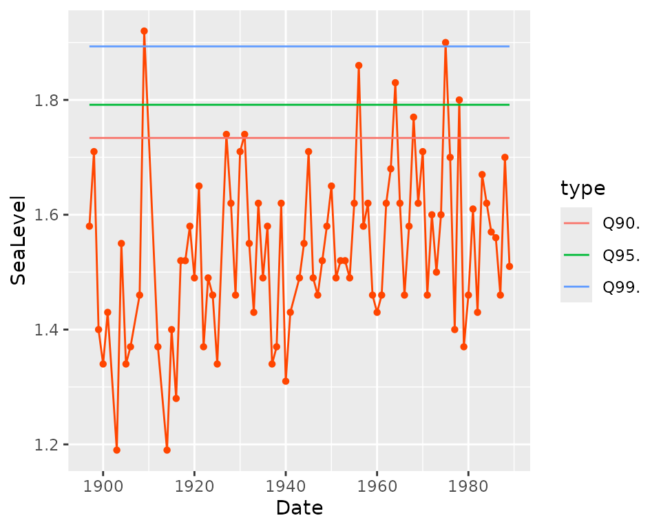

autoplot(fit1)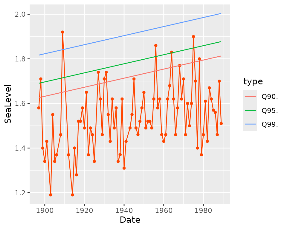

autoplot(fit2)

## Warning in quantile.TVGEV(object): 'x' includes TSVars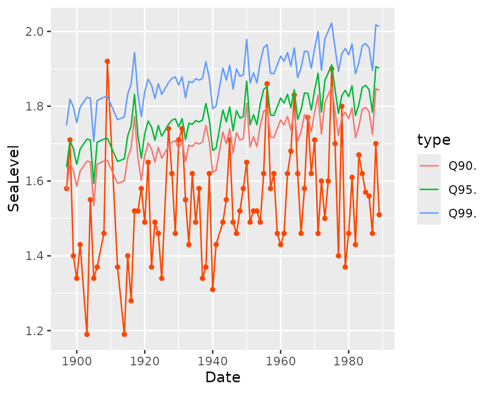

The autoplot method builds a ggplot object showing the observed response against the date along with the fitted quantiles for three levels of the probability of non-exceedance $p$, namely $p=0.90$, $p = 0.95$ and $p= 0.99$. These quantiles are those of the $\texttt{GEV}\{\mu(t),\,\sigma(t),\, \xi(t)\}$ distribution. When a timeseries covariate is used as for the object fit2, the quantiles are conditional on the value of the covariate for the corresponding year.

The methods coef, summary can be used to extract the vector $\widehat{\boldsymbol{\psi}}$ of estimated coefficients or get to a summary.

coef(fit2)

##         mu_0        mu_t1       mu_SOI      sigma_0         xi_0 
##  1.538642271  0.002113693  0.054532375  0.120730769 -0.150056860

summary(fit2)

## Call:
## TVGEV(data = df, date = "Date", response = "SeaLevel", design = polynomX(date = Date, 
##     degree = 1), loc = ~t1 + SOI)
## 
## Coefficients:
##             Estimate   Std. Error
## mu_0     1.538642271 0.0184556202
## mu_t1    0.002113693 0.0005189511
## mu_SOI   0.054532375 0.0196335168
## sigma_0  0.120730769 0.0101280359
## xi_0    -0.150056860 0.0666351631
## 
## Negative log-likelihood:
## -53.899

The output of summary suggests that the coefficient of $\texttt{SOI}(t)$ is significantly different from zero because in the row with label mu_SOI, the absolute value of the estimate $\widehat{\psi}^\mu_2$ is larger than twice the corresponding standard error. The trend coefficient mu_t1 is in meter by year so its value is 21.14 when expressed in centimeter by century, maybe a more suitable unit.

Note that the estimated GEV shape parameter in fit2 is fairly negative implying a finite upper end-point for the marginal GEV distributions.

Generalised residuals

The resid method of the "TVGEV" class computes the generalised residuals:

gr <- list()
gr[["0"]] <- autoplot(resid(fit0)) + ggtitle("fit0")
gr[["1"]] <- autoplot(resid(fit1)) + ggtitle("fit1")
gr[["2"]] <- autoplot(resid(fit2)) + ggtitle("fit2")

When a generalised residual falls far away in one of the two tails of the Gumbel distribution, it may be a good idea to check the influence of the corresponding observation on the fit.

When the variable SOI is used, the two years 1903 and 1914 have different residuals although they correspond to the same value of the sea level, because they correspond to different values of SOI. Although they correspond to severe coastal floodings, the largest sea levels in the dataset correspond to somewhat “normal” values of the residuals. This may mean that coastal flood defenses will have to be constantly improved.

Comparing nested models with likelihood-ratio tests

The anova method can be used to compare two nested models with Likelihood-Ratio test, for instance $M_0$ and $M_1$.

anova(fit0, fit1)

## Analysis of Deviance Table
## 
##      df deviance      W    Pr(>W)    
## fit0  3  -87.133                     
## fit1  4  -99.826 12.692 0.0003671 ***
## ---
## Signif. codes:  0 '***' 0.001 '**' 0.01 '*' 0.05 '.' 0.1 ' ' 1

So the likelihood-ratio test indicates that the linear trend term is strongly significant. Up to rounding, the maximised log-likelihoods are equal to those reported p. 113 in Coles (2001) book. We can similarly compare the two fitted models $M_1$ and $M_2$

anova(fit1, fit2)

## Analysis of Deviance Table
## 
##      df deviance      W   Pr(>W)   
## fit1  4  -99.826                   
## fit2  5 -107.798 7.9719 0.004751 **
## ---
## Signif. codes:  0 '***' 0.001 '**' 0.01 '*' 0.05 '.' 0.1 ' ' 1

So, as written p. 114 in Coles (2001) book: the effect of SOI is influential on annual maximum sea levels at Fremantle, even after the allowance for time variation. Again, the maximised log-likelihoods found here are in good agreement with that reported in the book.

Note that it is important to assess the effect of a timeseries covariates $z(t)$ such as $\texttt{SOI}(t)$ only when the effect of time has been taken into account. Without this precaution any covariate with a linear time trend would be found to be influential by a spurious regression effect. It may indeed be the case that the series $y(t)$ and $z(t)$ have a common trend.

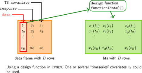
How TVGEV works

When a TVGEV function is created, the design argument can receive a call to a function that creates covariates $x_i(t)$ which are functions of the time i.e. of the variable specified in date. A data frame is created with its columns being the timeseries covariates $z(t)$ and the functions time $x_i(t)$. All these columns can be used in the lm-style formulas for the GEV parameters.

For instance the “design” matrix corresponding to the GEV location parameter $\mu$ can be extracted from the fitted model object.

 head(fit2$X[["loc"]])

##            (Intercept)        t1   SOI
## 1897-01-01           1 -72.99658 -0.67
## 1898-01-01           1 -71.99726  0.57
## 1899-01-01           1 -70.99795  0.16
## 1900-01-01           1 -69.99863 -0.65
## 1901-01-01           1 -68.99932  0.06
## 1903-01-01           1 -67.00068  0.47

This object could be coerced if needed to a timeseries object such as an object with class "xts" from the xts package.

Return levels or “prediction”

Return levels

Remind that the return levels are the quantiles of the GEV response $y(t)$. The corresponding probability $p$ is often converted into a return period $T$ in years according to the rule $p = 1 - 1/T$. For instance the so-called centennial return level for $T=100$ years corresponds to $p=0.99$ i.e., to a probability of exceedance of $0.01$.

Conditional return levels

As long as a TVGEV fitted model object involves only covariates that are functions of the time, the predict method only requires an argument newdate which defines the date(s) $t$ for which the quantiles are to be computed. For an object with no timeseries covariates, the value passed to this argument is usually a vector defining a future period: a set of years given by their beginning date. When timeseries covariates are used, one must give as well the value of these covariates for each predicted year. Then newdate must be a data frame with all the variables required for the prediction.

pred1 <- predict(fit1, newdate = c("2020-01-01", "2030-01-01"))
autoplot(pred1) + ggtitle("No TS covariate")

## Warning: Using `size` aesthetic for lines was deprecated in ggplot2 3.4.0.
## ℹ Please use `linewidth` instead.
## ℹ The deprecated feature was likely used in the NSGEV package.
##   Please report the issue at <https://github.com/IRSN/NSGEV/issues/>.
## This warning is displayed once every 8 hours.
## Call `lifecycle::last_lifecycle_warnings()` to see where this warning was
## generated.

## ~Date
## <environment: 0x55e99ffc8a98>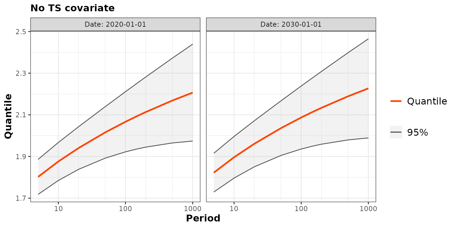

nd <- data.frame(Date = as.Date(c("2020-01-01", "2030-01-01")),
                 SOI = c(1.5, 2.1))
pred2 <- predict(fit2, newdate = nd)
autoplot(pred2) + ggtitle("Using the TS covariate `SOI`")

## ~Date + SOI
## <environment: 0x55e99c977840>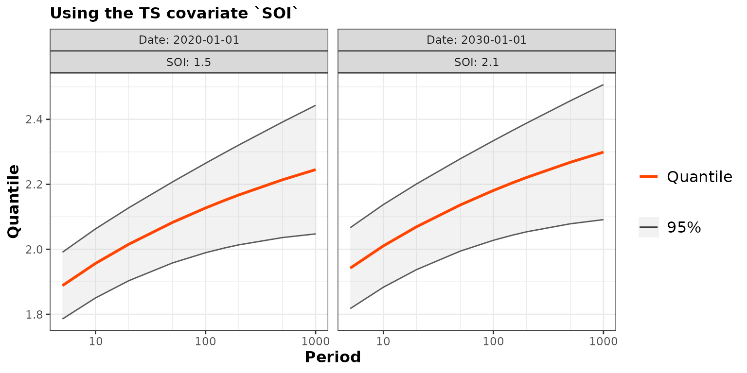

By default the confidence intervals on the return levels are obtained by using the “delta method”. Yet the confintMethod argument of the predict method can be used to get profile likelihood intervals instead. Partial matching can be used both for the argument and for its value: the choice "proflik" can be abbreviated as "prof" which is still well understood. Remind that the confidence intervals are approximate unless a very large sample is used. Still, profile likelihood intervals are known to have a better coverage those obtained by the delta method.

predProf1 <- predict(fit1, newdate = c("2020-01-01", "2030-01-01"),
                     conf = "prof", trace = 0)
autoplot(predProf1) + ggtitle("No TS covariate. Conf.: Prof. Lik ")

## ~Date
## <environment: 0x55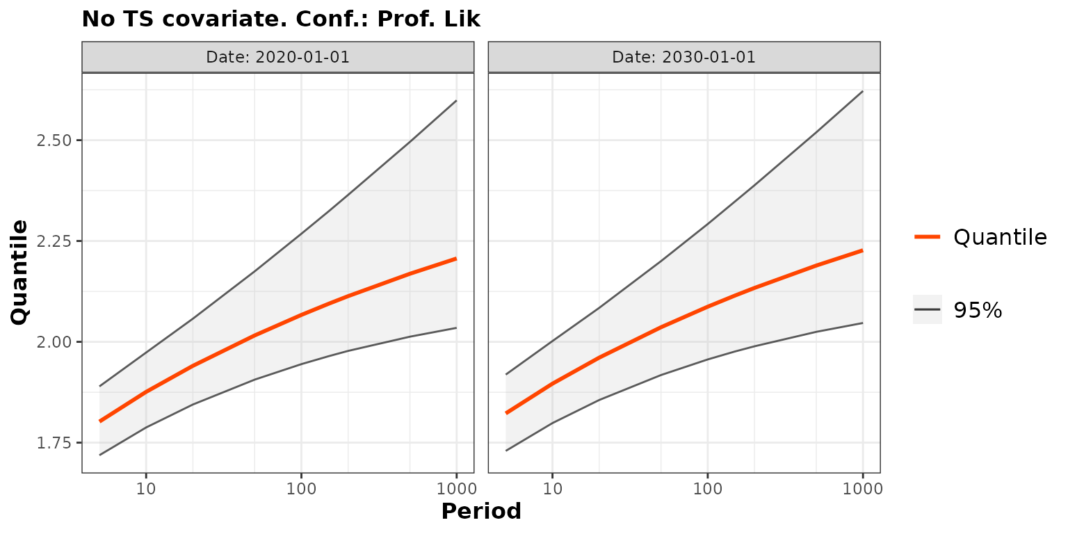e9a149d788>

nd <- data.frame(Date = as.Date(c("2020-01-01", "2030-01-01")),
                 SOI = c(1.5, 2.1))
predProf2 <- predict(fit2, newdate = nd, conf = "prof", trace = 0)
autoplot(predProf2) + ggtitle("Covariable TS `SOI`. Conf: Prof. Lik.")

## ~Date + SOI
## <environment: 0x55e9a2345d78>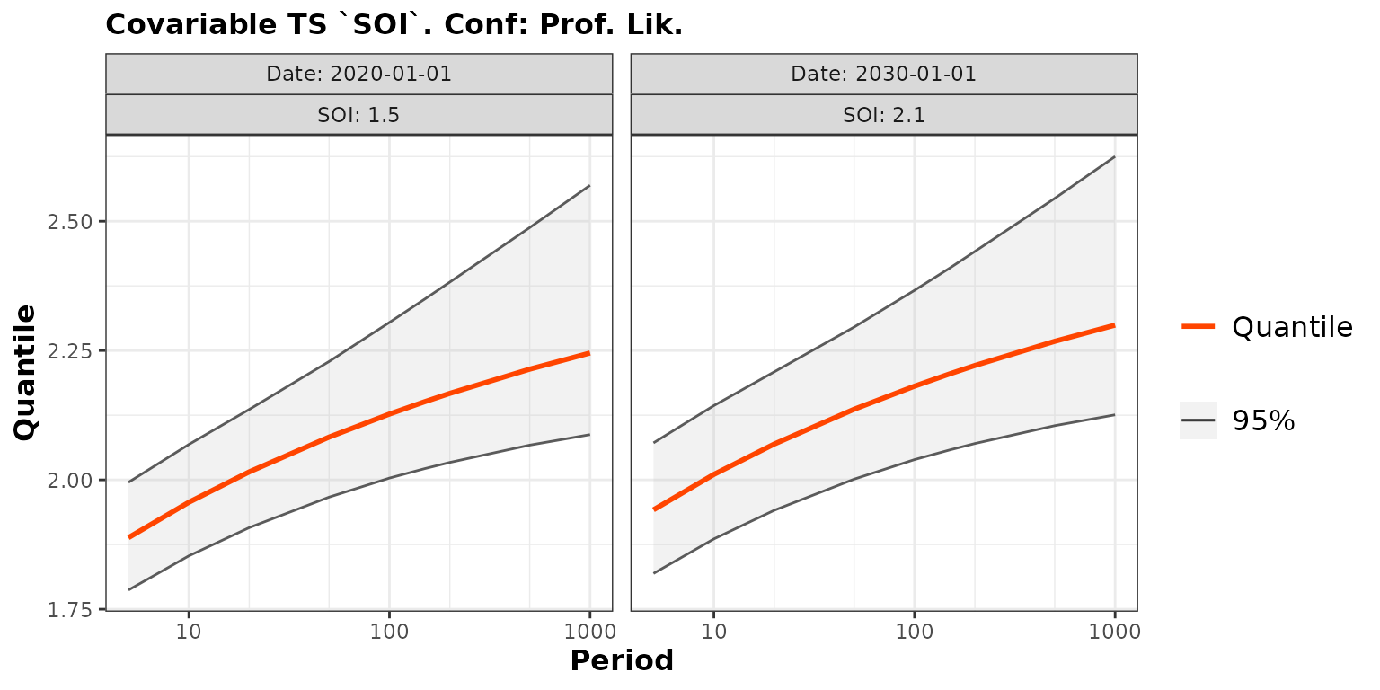

Note that the use of the SOI covariate leads to slightly narrower confidence intervals on the quantiles.

Remark In the previous code chunk trace = 0 was used to avoid a verbose output. A grid of return periods is used for the computation and for each return period, the confidence limits are actually obtained by using a constrained optimisation. When the trace argument is not zero, convergence diagnostics are printed. It may happen that the optimisation fails to converge.

Marginal return levels

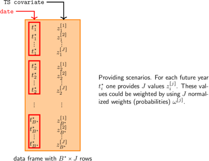
Rather than fixing a value for the covariates, one may want to “marginalise out” the return levels w.r.t the values of the covariate, or to “integrate out” these values, see Emma F. Eastoe and Jonathan A. Tawn (2009). The marginal return levels are not available yet but should be in a future version of the package. The return level corresponding to a future date of interest $t^\star$ average over a number of possible values $z^{[j]}$ or “scenarios” for the covariate $z(t^\star)$ that would be provided.

Limitations and possible extensions

For now the distribution of the maximum on a given period can not be computed when timeseries covariates are used.

The NSGEV package does not allow for models including latent variables. Such models can be used with INLA or rstan.

Appendix : using NAs for missing observations

Starting form the fremantle data frame, we can build a new data frame containing all the years between the first and the last year of the original data frame. The merge method can be used for this aim, with the Date as key. All the columns except Date will contain NAs for the missing years.

Date = seq(from = df$Date[1], to = df$Date[nrow(df)], by = "year")
dfNA <- merge(df, data.frame(Date), by = "Date", all.y = TRUE)
summary(dfNA)

##       Date                 Year         SeaLevel          SOI          
##  Min.   :1897-01-01   Min.   :1897   Min.   :1.190   Min.   :-1.78000  
##  1st Qu.:1920-01-01   1st Qu.:1923   1st Qu.:1.460   1st Qu.:-0.44500  
##  Median :1943-01-01   Median :1946   Median :1.520   Median : 0.06000  
##  Mean   :1943-01-01   Mean   :1945   Mean   :1.538   Mean   :-0.03267  
##  3rd Qu.:1966-01-01   3rd Qu.:1968   3rd Qu.:1.620   3rd Qu.: 0.37250  
##  Max.   :1989-01-01   Max.   :1989   Max.   :1.920   Max.   : 2.12000  
##                       NA's   :7      NA's   :7       NA's   :7

Then we can fit the same TVGEV model as before

fit2NA <- TVGEV(data = dfNA, response = "SeaLevel", date = "Date",
                design = polynomX(date = Date, degree = 1),
                loc = ~ t1 + SOI)

We see that the results of the estimation with NA observations are identical to those obtained with the missing years.

References

Coles, Suart. 2001. An Introduction to Statistical Modeling of Extreme Values. Springer. https://doi.org/10.1007/978-1-4471-3675-0.

Emma F. Eastoe and Jonathan A. Tawn. 2009. “Modelling Non-Stationary Extremes with Application to Surface Level Ozone.” Applied Statistics 58: 25–45. https://doi.org/10.1111/j.1467-9876.2008.00638.x.