Generalised Residuals for a TVGEV Model — residuals.TVGEV • NSGEV

Generalised Residuals for a TVGEV model.

# S3 method for class 'TVGEV'
residuals(object, type = c("gumbel", "exp", "unif"), ...)

Arguments

object: A TVGEV object.
type: The approximate distribution wanted. The choices c("unif", "exp", "gumbel") correspond to the standard uniform, the standard exponential and the standard Gumbel distributions. Partial matching is allowed.
...: Not used yet.

Value

A vector of generalised residuals which should approximately be independent and approximately follow the target distribution: standard Gumbel, standard exponential or standard uniform, depending on the value of type.

Details

The generalised residuals are obtained by applying to each observation $y_b$ an increasing function depending on the (estimated) GEV parameters $\boldsymbol{\theta}_b$ .

Note

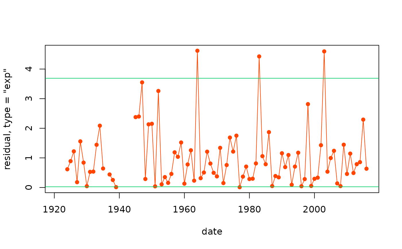
The upper 95% quantile of the standard Gumbel and the standard exponential is close to $3$ which can be used to gauge "large residuals". Using type = "gumbel" seems better to diagnose abnormally small residuals as may result from abnormally small block maxima.

References

Cox, D.R. and Snell E.J. (1968) "A General Definition of Residuals". JRSS Ser. B, 30(2), pp. 248-275, doi:10.1111/j.2517-6161.1968.tb00724.x .

Katz, R.W. and Parlange, M. B. and Naveau, P. (2002) "Statistics of extremes in hydrology", Advances in Water Resources, 25(8), pp. 1287-1304, doi:10.1016/S0309-1708(02)00056-8 .

Panagoulia, D. and Economou, P. and Caroni, C. (2014) "Stationary and Nonstationary Generalized Extreme Value Modelling of Extreme Precipitation over a Mountainous Area under Climate Change". Environmetrics 25(1), pp. 29-43, doi:10.1002/env.2252 .

Examples

df <- within(TXMax_Dijon, Date <- as.Date(sprintf("%4d-01-01", Year)))
tv <- TVGEV(data = df, response = "TXMax", date = "Date",
            design = breaksX(date = Date, breaks = "1970-01-01", degree = 1),
            loc = ~ t1 + t1_1970)
e <- resid(tv)
plot(e)

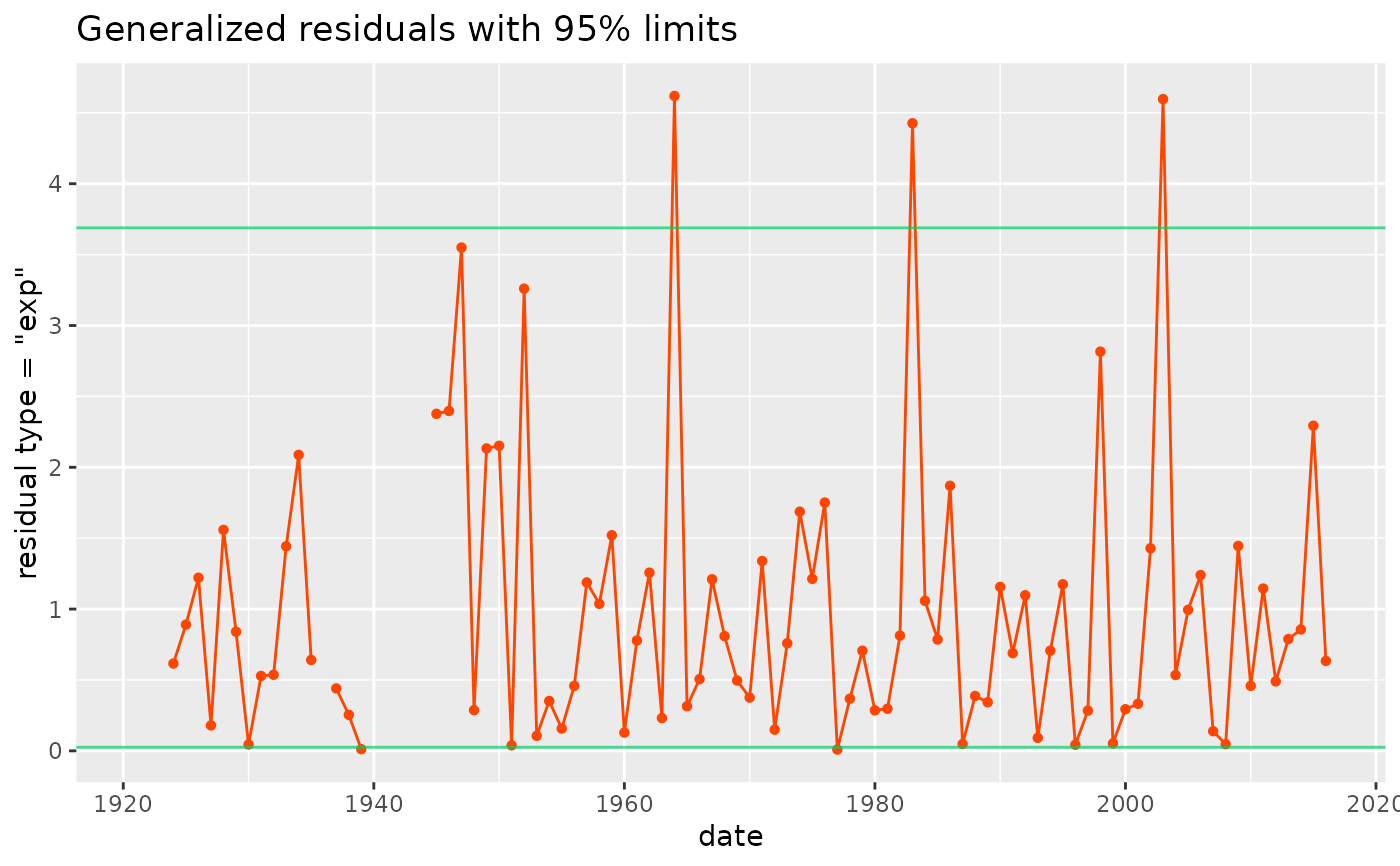
## ggplot alternative
autoplot(e)
#> Warning: Removed 3 rows containing missing values or values outside the scale range
#> (`geom_line()`).
#> Warning: Removed 9 rows containing missing values or values outside the scale range
#> (`geom_point()`).

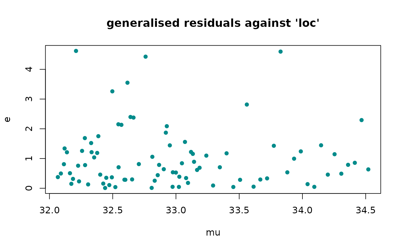
## plot the residual against the fitted location. Use 'as.numeric'
## on the residuals to build a similar ggplot
mu <- tv$theta[ , "loc"]
plot(mu, e, type = "p", pch = 16, col = "darkcyan",
     main = "generalised residuals against 'loc'")