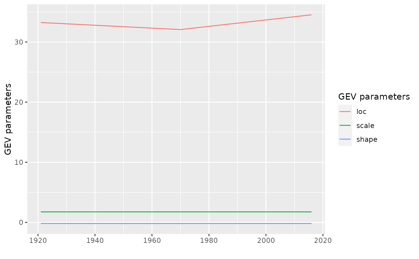
Time-Plot of bts Objects for Block Time Series

Time-plot of a bts object.

# S3 method for bts
plot(x, y, gg = TRUE, col1 = "darkgray", facets = FALSE, ...)

# S3 method for bts
lines(x, y, col1 = "gray", alpha = NULL, ...)

Arguments

x

A bts object representing a Block Time Series, such as the GEV parameters of a TVGEV model.

y

Not used yet.

gg

Logical. If TRUE, a ggplot plot will be drawn and returned by the function. If FALSE a standard plot is shown and the function returns nothing.

col1

A colour which is used in the case where x has more than 12 columns. In this case, all the curves are drawn using the colour col1.

facets

Logical. If True, the columns of x will be shown each in a facet. Only works if the number of columns is between 2 and 12.

...

Further parameter passed to graphical functions.

alpha

Level of opacity. By default, the opacity is lowered when the number of time series is increased.

Value

An object inheriting from "ggplot" if gg

is TRUE.

Note

When a plot is built with gg = TRUE, using the lines method later will have no effect, because this method is designed to work on standard graphics, and not with graphics produced by ggplot2.

See also

quantile.TVGEV, mean.TVGEV for some examples of "bts" objects and their use in plots.

Examples

example(TVGEV)
#> 
#> TVGEV> ## transform a numeric year into a date
#> TVGEV> df <- within(TXMax_Dijon, Date <- as.Date(sprintf("%4d-01-01", Year)))
#> 
#> TVGEV> df0 <- subset(df, !is.na(TXMax))
#> 
#> TVGEV> ## fit a TVGEV model. Only the location parameter is TV.
#> TVGEV> t1 <- system.time(
#> TVGEV+     res1 <- TVGEV(data = df, response = "TXMax", date = "Date",
#> TVGEV+                   design = breaksX(date = Date, breaks = "1970-01-01", degree = 1),
#> TVGEV+                   loc = ~ t1 + t1_1970))
#> 
#> TVGEV> ## The same using "nloptr" optimisation.
#> TVGEV> t2 <- system.time(
#> TVGEV+     res2 <- TVGEV(data = df, response = "TXMax", date = "Date",
#> TVGEV+                   design = breaksX(date = Date, breaks = "1970-01-01", degree = 1),
#> TVGEV+                   loc = ~ t1 + t1_1970,
#> TVGEV+                   estim = "nloptr",
#> TVGEV+                   parTrack = TRUE))
#> 
#> TVGEV> ## use extRemes::fevd the required variables need to be added to the data frame
#> TVGEV> ## passed as 'data' argument
#> TVGEV> t0 <- system.time({
#> TVGEV+    df0.evd <- cbind(df0, breaksX(date = df0$Date, breaks = "1970-01-01",
#> TVGEV+                     degree = 1));
#> TVGEV+    res0 <- fevd(x = df0.evd$TXMax, data = df0.evd, loc = ~ t1 + t1_1970)
#> TVGEV+  })
#> 
#> TVGEV> ## compare estimate and negative log-liks
#> TVGEV> cbind("fevd" = res0$results$par,
#> TVGEV+       "TVGEV_optim" = res1$estimate,
#> TVGEV+       "TVGEV_nloptr" = res2$estimate)
#>              fevd TVGEV_optim TVGEV_nloptr
#> mu0   32.06678895 32.06638460  32.06679233
#> mu1   -0.02391857 -0.02392656  -0.02391860
#> mu2    0.07727041  0.07728411   0.07727031
#> scale  1.75585289  1.75541862   1.75585346
#> shape -0.18130928 -0.18112018  -0.18130938
#> 
#> TVGEV> cbind("fevd" = res0$results$value,
#> TVGEV+       "VGEV_optim" = res1$negLogLik,
#> TVGEV+       "TVGEV_nloptr" = res2$negLogLik)
#>          fevd VGEV_optim TVGEV_nloptr
#> [1,] 177.2014   177.2014     177.2014
#> 
#> TVGEV> ## ====================================================================
#> TVGEV> ## use a loop on plausible break years. The fitted models
#> TVGEV> ## are stored within a list
#> TVGEV> ## ====================================================================
#> TVGEV> 
#> TVGEV> ## Not run: 
#> TVGEV> ##D 
#> TVGEV> ##D     yearBreaks <- c(1940, 1950, 1955, 1960:2000, 2005, 2010)
#> TVGEV> ##D     res <- list()
#> TVGEV> ##D 
#> TVGEV> ##D     for (ib in seq_along(yearBreaks)) {
#> TVGEV> ##D         d <- sprintf("%4d-01-01", yearBreaks[[ib]])
#> TVGEV> ##D         floc <- as.formula(sprintf("~ t1 + t1_%4d", yearBreaks[[ib]]))
#> TVGEV> ##D         res[[d]] <- TVGEV(data = df, response = "TXMax", date = "Date",
#> TVGEV> ##D         design = breaksX(date = Date, breaks = d, degree = 1),
#> TVGEV> ##D         loc = floc)
#> TVGEV> ##D     }
#> TVGEV> ##D 
#> TVGEV> ##D     ## [continuing...] ]find the model with maximum likelihood, and plot
#> TVGEV> ##D     ## something like a profile likelihood for the break date considered
#> TVGEV> ##D     ## as a new parameter. However, the model is not differentiable w.r.t.
#> TVGEV> ##D     ## the break! 
#> TVGEV> ##D 
#> TVGEV> ##D     ll <- sapply(res, logLik)
#> TVGEV> ##D     plot(yearBreaks, ll, type = "o", pch = 21, col = "orangered",
#> TVGEV> ##D          lwd = 2, bg = "gold", xlab = "break", ylab = "log-lik")
#> TVGEV> ##D     grid()
#> TVGEV> ##D     iMax <- which.max(ll)
#> TVGEV> ##D     abline(v = yearBreaks[iMax])
#> TVGEV> ##D     abline(h = ll[iMax] - c(0, qchisq(0.95, df = 1) /2),
#> TVGEV> ##D            col = "SpringGreen3", lwd = 2)
#> TVGEV> ##D 
#> TVGEV> ## End(Not run)
#> TVGEV> 
#> TVGEV> 
#> TVGEV> 
plot(coef(res1, type = "theta"))