This function provides some indications on the influence of a
specific observation used in the fit of a TVGEV object. For
several candidate values of the chosen observation, a TVGEV
is re-fitted with the observed value replaced by the candidate
value, and the quantity of interest as defined by what is
computed.
Arguments
- model
A
TVGEVobject.- what
A function with one argument
objectdefining or extracting the (numeric) quantity for which the influence is to be analysed. So,objectmust be aTVGEVobject. See Examples. This function can return numeric vector in which case several influence curves will be computed. It is then wise to make the function return a vector with named elements.- which
Identifies the observation which influence will be analysed. Can be: an integer giving the observation, the character
"min", the character"max", a character that can be coerced to a date, or an object with class"Date"that identifies the observation. This argument must define an observation existing in the data frame used to create the object. So it can not be used e.g. to define a future date.- how
Character specifying the type of (finite-sample) influence curve to use. For now only the only possibility is
"replace", see Section 2.1 of the book by Hampel et al (1996). The chosen observation is replaced by a value \(x\) and the quantity of interest is computed for each value of \(x\).- ...
Not used.
Value
A named list of vectors. The element obsValue
contains the candidate values for the chosen observation and
statValue contains the corresponding values of the
specific statistic defined with what.
Details
By suitably defining the function what, one can trace e.g.,
the estimate of a quantile with given probability, the
corresponding upper confidence limit, the upper end-point of the
distribution, ... and more.
Note
For TVGEV models with a positive GEV shape, the
smallest observation may have a strong influence on the
result, even if the model is stationary.
References
Hampel, F.R., Ronchetti, E.M., Rousseeuw, P.J. and Stahel W.A. (1996) Robust Statistics: The Approach Based on Influence Functions. Wiley.
Examples
example(TVGEV)
#>
#> TVGEV> ## transform a numeric year into a date
#> TVGEV> df <- within(TXMax_Dijon, Date <- as.Date(sprintf("%4d-01-01", Year)))
#>
#> TVGEV> df0 <- subset(df, !is.na(TXMax))
#>
#> TVGEV> ## fit a TVGEV model. Only the location parameter is TV.
#> TVGEV> t1 <- system.time(
#> TVGEV+ res1 <- TVGEV(data = df, response = "TXMax", date = "Date",
#> TVGEV+ design = breaksX(date = Date, breaks = "1970-01-01", degree = 1),
#> TVGEV+ loc = ~ t1 + t1_1970))
#>
#> TVGEV> ## The same using "nloptr" optimisation.
#> TVGEV> t2 <- system.time(
#> TVGEV+ res2 <- TVGEV(data = df, response = "TXMax", date = "Date",
#> TVGEV+ design = breaksX(date = Date, breaks = "1970-01-01", degree = 1),
#> TVGEV+ loc = ~ t1 + t1_1970,
#> TVGEV+ estim = "nloptr",
#> TVGEV+ parTrack = TRUE))
#>
#> TVGEV> ## use extRemes::fevd the required variables need to be added to the data frame
#> TVGEV> ## passed as 'data' argument
#> TVGEV> t0 <- system.time({
#> TVGEV+ df0.evd <- cbind(df0, breaksX(date = df0$Date, breaks = "1970-01-01",
#> TVGEV+ degree = 1));
#> TVGEV+ res0 <- fevd(x = df0.evd$TXMax, data = df0.evd, loc = ~ t1 + t1_1970)
#> TVGEV+ })
#>
#> TVGEV> ## compare estimate and negative log-liks
#> TVGEV> cbind("fevd" = res0$results$par,
#> TVGEV+ "TVGEV_optim" = res1$estimate,
#> TVGEV+ "TVGEV_nloptr" = res2$estimate)
#> fevd TVGEV_optim TVGEV_nloptr
#> mu0 32.06678895 32.06638460 32.06679282
#> mu1 -0.02391857 -0.02392656 -0.02391856
#> mu2 0.07727041 0.07728411 0.07727061
#> scale 1.75585289 1.75541862 1.75585353
#> shape -0.18130928 -0.18112018 -0.18131041
#>
#> TVGEV> cbind("fevd" = res0$results$value,
#> TVGEV+ "VGEV_optim" = res1$negLogLik,
#> TVGEV+ "TVGEV_nloptr" = res2$negLogLik)
#> fevd VGEV_optim TVGEV_nloptr
#> [1,] 177.2014 177.2014 177.2014
#>
#> TVGEV> ## ====================================================================
#> TVGEV> ## use a loop on plausible break years. The fitted models
#> TVGEV> ## are stored within a list
#> TVGEV> ## ====================================================================
#> TVGEV>
#> TVGEV> ## Not run:
#> TVGEV> ##D
#> TVGEV> ##D yearBreaks <- c(1940, 1950, 1955, 1960:2000, 2005, 2010)
#> TVGEV> ##D res <- list()
#> TVGEV> ##D
#> TVGEV> ##D for (ib in seq_along(yearBreaks)) {
#> TVGEV> ##D d <- sprintf("%4d-01-01", yearBreaks[[ib]])
#> TVGEV> ##D floc <- as.formula(sprintf("~ t1 + t1_%4d", yearBreaks[[ib]]))
#> TVGEV> ##D res[[d]] <- TVGEV(data = df, response = "TXMax", date = "Date",
#> TVGEV> ##D design = breaksX(date = Date, breaks = d, degree = 1),
#> TVGEV> ##D loc = floc)
#> TVGEV> ##D }
#> TVGEV> ##D
#> TVGEV> ##D ## [continuing...] ]find the model with maximum likelihood, and plot
#> TVGEV> ##D ## something like a profile likelihood for the break date considered
#> TVGEV> ##D ## as a new parameter. However, the model is not differentiable w.r.t.
#> TVGEV> ##D ## the break!
#> TVGEV> ##D
#> TVGEV> ##D ll <- sapply(res, logLik)
#> TVGEV> ##D plot(yearBreaks, ll, type = "o", pch = 21, col = "orangered",
#> TVGEV> ##D lwd = 2, bg = "gold", xlab = "break", ylab = "log-lik")
#> TVGEV> ##D grid()
#> TVGEV> ##D iMax <- which.max(ll)
#> TVGEV> ##D abline(v = yearBreaks[iMax])
#> TVGEV> ##D abline(h = ll[iMax] - c(0, qchisq(0.95, df = 1) /2),
#> TVGEV> ##D col = "SpringGreen3", lwd = 2)
#> TVGEV> ##D
#> TVGEV> ## End(Not run)
#> TVGEV>
#> TVGEV>
#> TVGEV>
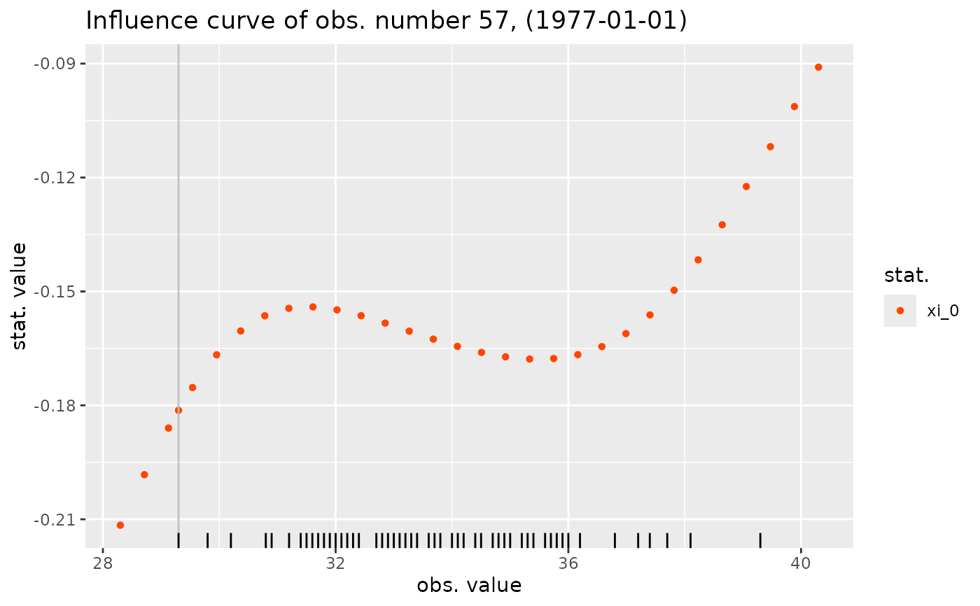
influ <- influence(res2, which = "min")
autoplot(influ)
#> Warning: Removed 9 rows containing missing values or values outside the scale range
#> (`geom_rug()`).
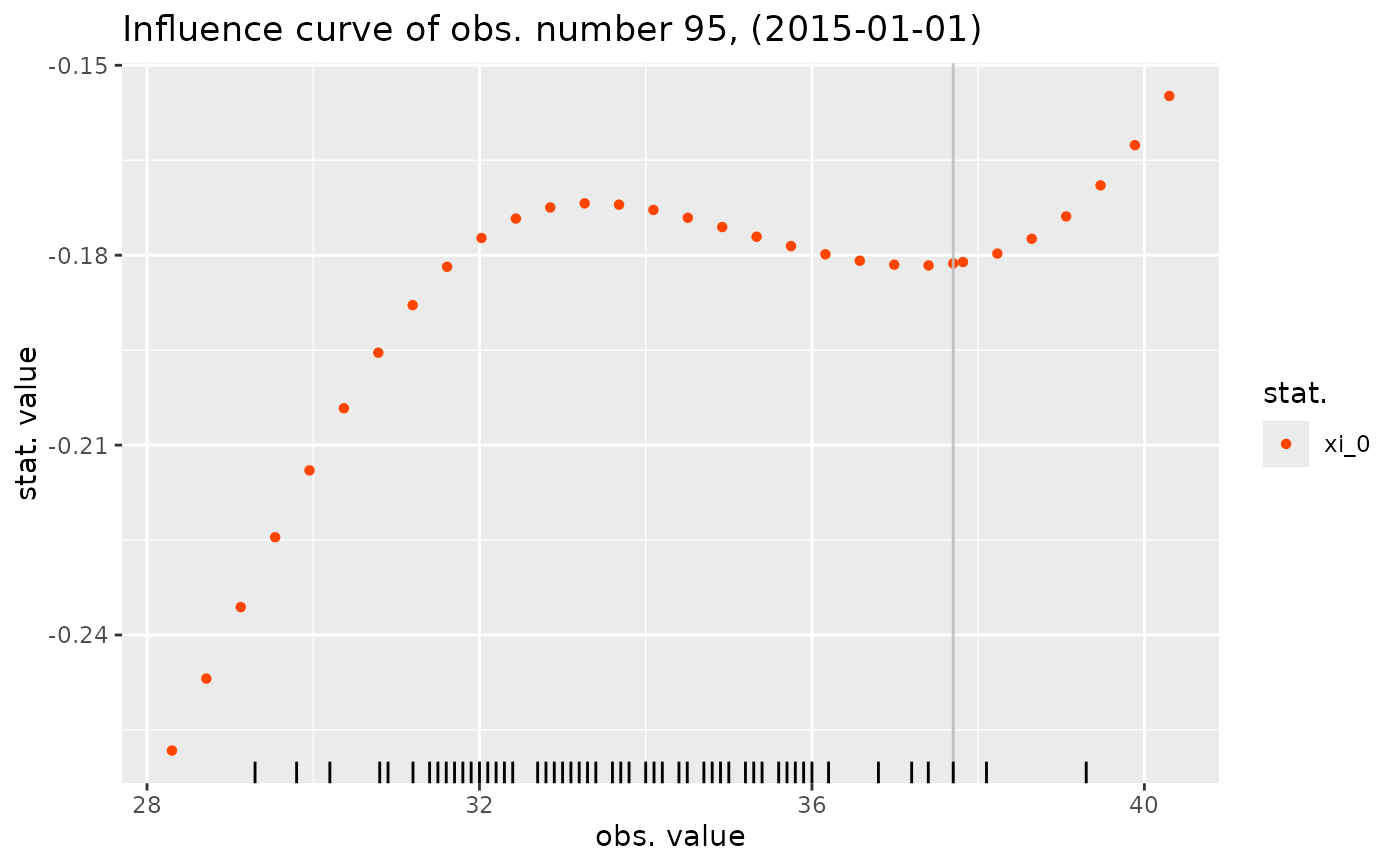
 influ <- influence(res2, which = as.Date("2015-01-01"))
autoplot(influ)
#> Warning: Removed 9 rows containing missing values or values outside the scale range
#> (`geom_rug()`).
influ <- influence(res2, which = as.Date("2015-01-01"))
autoplot(influ)
#> Warning: Removed 9 rows containing missing values or values outside the scale range
#> (`geom_rug()`).
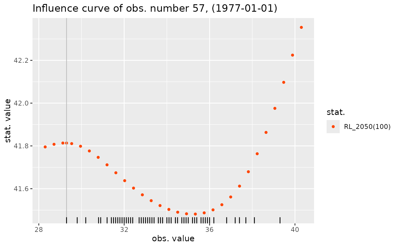
 RL_2050 <- function(model) {
c("RL_2050(100)" = quantile(model, prob = 0.99, date = "2050-01-01")[1])
}
influence(res2, what = RL_2050) |> autoplot()
#> Warning: Removed 9 rows containing missing values or values outside the scale range
#> (`geom_rug()`).
RL_2050 <- function(model) {
c("RL_2050(100)" = quantile(model, prob = 0.99, date = "2050-01-01")[1])
}
influence(res2, what = RL_2050) |> autoplot()
#> Warning: Removed 9 rows containing missing values or values outside the scale range
#> (`geom_rug()`).
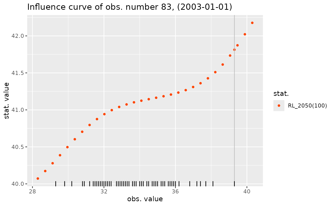
 influence(res2, what = RL_2050, which = "2003-01-01") |> autoplot()
#> Warning: Removed 9 rows containing missing values or values outside the scale range
#> (`geom_rug()`).
influence(res2, what = RL_2050, which = "2003-01-01") |> autoplot()
#> Warning: Removed 9 rows containing missing values or values outside the scale range
#> (`geom_rug()`).
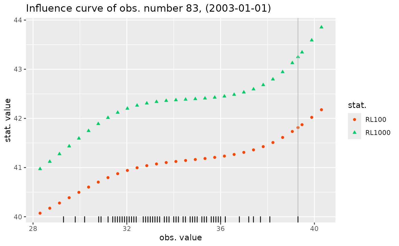
 RLs_2050 <- function(model) {
res <- c(quantile(model, prob = 0.99, date = "2050-01-01")[1],
quantile(model, prob = 0.999, date = "2050-01-01")[1])
names(res) <- paste0("RL", c(100, 1000))
res
}
influ <- influence(res2, what = RLs_2050, which = "2003-01-01")
autoplot(influ)
#> Warning: Removed 9 rows containing missing values or values outside the scale range
#> (`geom_rug()`).
RLs_2050 <- function(model) {
res <- c(quantile(model, prob = 0.99, date = "2050-01-01")[1],
quantile(model, prob = 0.999, date = "2050-01-01")[1])
names(res) <- paste0("RL", c(100, 1000))
res
}
influ <- influence(res2, what = RLs_2050, which = "2003-01-01")
autoplot(influ)
#> Warning: Removed 9 rows containing missing values or values outside the scale range
#> (`geom_rug()`).