Compute TVGEV Densities or Cumulative Distribution Functions

Compute TVGEV densities or Cumulative Distribution Functions.

# S3 method for TVGEV
density(x, xValue = NULL, date = NULL, psi = NULL, log = FALSE, ...)

# S3 method for TVGEV
cdf(x, qValue = NULL, date = NULL, psi = NULL, log = FALSE, ...)

Arguments

x: A TVGEV object.
xValue: Vector of quantiles at which the GEV densities will be evaluated. By default, a grid of value is found with coverage probability > 0.001 for each observation.
date: An object that can be coerced to the class"Date" giving the date of the blocks for which the density will be evaluated. By default, three dates are selected in the date vector attached to x.
psi: Vector of model coefficients. By default, the vector of estimated coefficients in x is used.
log: Logical. If TRUE the log-density is returned.
...: Other arguments to be passed to dGEV or pGEV.
qValue: xValue Vector of probabilities at which the GEV densities will be evaluated. By default, a grid of value from 0.0 to 1.0 is used. for each observation.

Value

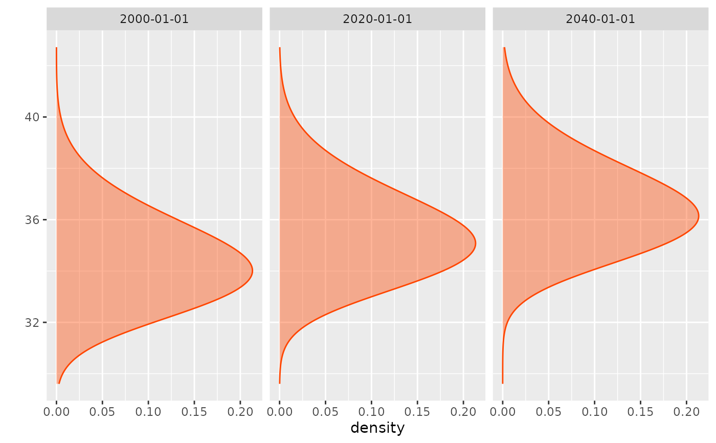
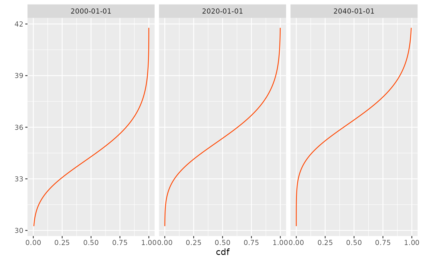
An oject with class "bfts". This is mainly a matrix with one row by date. Rather than providing a time-plot of each column (as would be done for a "bts" object), the plot method plots the density or cdf function for a small number of dates. Unless the number of dates is 1, the functions are plotted with the x-y axes flipped in order to enhance the time-varying feature of the model.

Examples

example(TVGEV)
#> 
#> TVGEV> ## transform a numeric year into a date
#> TVGEV> df <- within(TXMax_Dijon, Date <- as.Date(sprintf("%4d-01-01", Year)))
#> 
#> TVGEV> df0 <- subset(df, !is.na(TXMax))
#> 
#> TVGEV> ## fit a TVGEV model. Only the location parameter is TV.
#> TVGEV> t1 <- system.time(
#> TVGEV+     res1 <- TVGEV(data = df, response = "TXMax", date = "Date",
#> TVGEV+                   design = breaksX(date = Date, breaks = "1970-01-01", degree = 1),
#> TVGEV+                   loc = ~ t1 + t1_1970))
#> 
#> TVGEV> ## The same using "nloptr" optimisation.
#> TVGEV> t2 <- system.time(
#> TVGEV+     res2 <- TVGEV(data = df, response = "TXMax", date = "Date",
#> TVGEV+                   design = breaksX(date = Date, breaks = "1970-01-01", degree = 1),
#> TVGEV+                   loc = ~ t1 + t1_1970,
#> TVGEV+                   estim = "nloptr",
#> TVGEV+                   parTrack = TRUE))
#> 
#> TVGEV> ## use extRemes::fevd the required variables need to be added to the data frame
#> TVGEV> ## passed as 'data' argument
#> TVGEV> t0 <- system.time({
#> TVGEV+    df0.evd <- cbind(df0, breaksX(date = df0$Date, breaks = "1970-01-01",
#> TVGEV+                     degree = 1));
#> TVGEV+    res0 <- fevd(x = df0.evd$TXMax, data = df0.evd, loc = ~ t1 + t1_1970)
#> TVGEV+  })
#> 
#> TVGEV> ## compare estimate and negative log-liks
#> TVGEV> cbind("fevd" = res0$results$par,
#> TVGEV+       "TVGEV_optim" = res1$estimate,
#> TVGEV+       "TVGEV_nloptr" = res2$estimate)
#>              fevd TVGEV_optim TVGEV_nloptr
#> mu0   32.06678895 32.06638460  32.06679233
#> mu1   -0.02391857 -0.02392656  -0.02391860
#> mu2    0.07727041  0.07728411   0.07727031
#> scale  1.75585289  1.75541862   1.75585346
#> shape -0.18130928 -0.18112018  -0.18130938
#> 
#> TVGEV> cbind("fevd" = res0$results$value,
#> TVGEV+       "VGEV_optim" = res1$negLogLik,
#> TVGEV+       "TVGEV_nloptr" = res2$negLogLik)
#>          fevd VGEV_optim TVGEV_nloptr
#> [1,] 177.2014   177.2014     177.2014
#> 
#> TVGEV> ## ====================================================================
#> TVGEV> ## use a loop on plausible break years. The fitted models
#> TVGEV> ## are stored within a list
#> TVGEV> ## ====================================================================
#> TVGEV> 
#> TVGEV> ## Not run: 
#> TVGEV> ##D 
#> TVGEV> ##D     yearBreaks <- c(1940, 1950, 1955, 1960:2000, 2005, 2010)
#> TVGEV> ##D     res <- list()
#> TVGEV> ##D 
#> TVGEV> ##D     for (ib in seq_along(yearBreaks)) {
#> TVGEV> ##D         d <- sprintf("%4d-01-01", yearBreaks[[ib]])
#> TVGEV> ##D         floc <- as.formula(sprintf("~ t1 + t1_%4d", yearBreaks[[ib]]))
#> TVGEV> ##D         res[[d]] <- TVGEV(data = df, response = "TXMax", date = "Date",
#> TVGEV> ##D         design = breaksX(date = Date, breaks = d, degree = 1),
#> TVGEV> ##D         loc = floc)
#> TVGEV> ##D     }
#> TVGEV> ##D 
#> TVGEV> ##D     ## [continuing...] ]find the model with maximum likelihood, and plot
#> TVGEV> ##D     ## something like a profile likelihood for the break date considered
#> TVGEV> ##D     ## as a new parameter. However, the model is not differentiable w.r.t.
#> TVGEV> ##D     ## the break! 
#> TVGEV> ##D 
#> TVGEV> ##D     ll <- sapply(res, logLik)
#> TVGEV> ##D     plot(yearBreaks, ll, type = "o", pch = 21, col = "orangered",
#> TVGEV> ##D          lwd = 2, bg = "gold", xlab = "break", ylab = "log-lik")
#> TVGEV> ##D     grid()
#> TVGEV> ##D     iMax <- which.max(ll)
#> TVGEV> ##D     abline(v = yearBreaks[iMax])
#> TVGEV> ##D     abline(h = ll[iMax] - c(0, qchisq(0.95, df = 1) /2),
#> TVGEV> ##D            col = "SpringGreen3", lwd = 2)
#> TVGEV> ##D 
#> TVGEV> ## End(Not run)
#> TVGEV> 
#> TVGEV> 
#> TVGEV> 
d <- density(res1, date = c("2000-01-01", "2020-01-01", "2040-01-01"))
F <- cdf(res1, date = c("2000-01-01", "2020-01-01", "2040-01-01"))
plot(d, fill = TRUE)

plot(F)

Compute TVGEV Densities or Cumulative Distribution Functions

Arguments

Value

See also

Examples