Return Levels for NSGEV and TVGEV objects

Return Levels for NSGEV and TVGEV Objects.

RL(
  model,
  period,
  data = NULL,
  date = NULL,
  psi = NULL,
  w = 1,
  type = c("exceed", "average"),
  sampleData = FALSE,
  deriv = FALSE,
  rhoMin = NULL,
  rhoMax = NULL,
  plot = FALSE
)

Arguments

model: A NSGEV or TVGEV object.
period: The Return period. Should be understood as an integer multiple of the block duration w, and will be rounded else. In some cases period must not exceed the number of rows in data, see Details.
data: To be used only when model has class "NSGEV". A data frame containing covariates for the model. By default, the data frame attached to model is used.
date: To be used only when model has class "TVGEV". A vector that can be coerced to the "Date" class. By default, the date attached to model is used.
psi: Vector of coefficients. By default, the vector of coefficients of the model is used.
w: Numeric scalar: duration of the blocks.
type: The type of RL wanted, see Details.
sampleData: Logical. Only used for NSGEV objects. If TRUE, the rows of data are assumed to form a sample of the distribution of the covariates and will be re-sampled.
deriv: Logical. If TRUE the gradient of the RL w.r.t the model parameters is returned.
rhoMin: Minimal value for the evaluation of the function in the zero-finding step when type is "exceed". This should be used if the zero is not found with the default value, which can be diagnosed then with plot = TRUE.
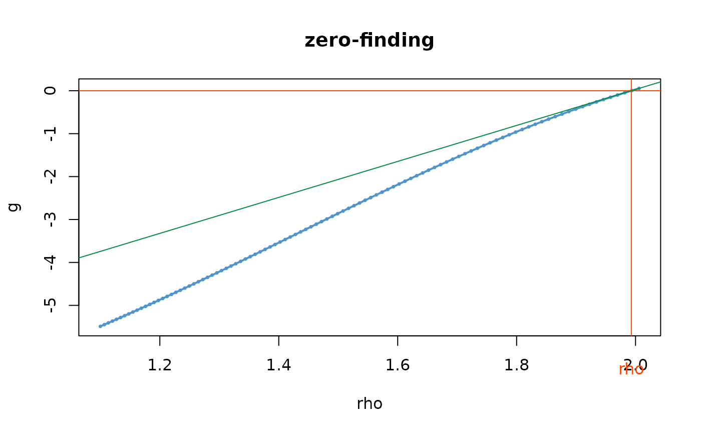
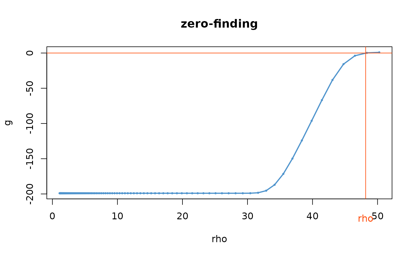
rhoMax: Maximal value for the evaluation of the function in the zero-finding step when type is "exceed". This should be used if the zero is not found with the default value, which can be diagnosed then with plot = TRUE.
plot: Logical. If type is "expect", a plot is shown to check the results of the zero-finding step.

Value

The numeric value of the Return Level.

Details

In all cases, the GEV parameters \(\boldsymbol{\theta}_b\) corresponding to the model and the rows \(b\) of data are computed. When sampleData is TRUE the rows are assumed to form a sample of the target distribution of the GEV parameters and will be re-sampled, so the result will change in successive calls. When instead sampleData is FALSE, the rows of data are considered as the values of the covariates that will be observed in the next 'future' blocks. Then the Return period can not be greater than the number of rows in 'data'.

When type is "average", the RL is computed for each value of the GEV parameter and the result is simply the mean of the computed RLs.
When type is "exceed" the RL is the value \(\rho\) for which the number of exeedances over \(\rho\) has unit expectation, as proposed by Parey et al. This value is found by computing the expectation and solving a non-linear equation in \(\rho\) with uniroot function.

Caution

For now, period can only be a numeric vector with length 1.

References

Parey S., Hoang T.T.H., Dacunha-Castelle D. (2007) "Different ways to compute temperature return levels in the climate change context". Environmetrics, 21, pp. 698-718.

Author

Yves Deville

Examples

## =================
## NSGEV examples
## =================
example(NSGEV)
#> 
#> NSGEV> df <- data.frame(t = 1:10)
#> 
#> NSGEV> ## built a model with given coefficients
#> NSGEV> psi <- c("alpha" = 1, "beta" = 0.01, "delta" = 0.6, "xi" = 0.06)
#> 
#> NSGEV> ns0 <- NSGEV(formulas = list("loc" = ~ alpha + beta * t, "scale" = ~ delta, "shape" = ~ xi),
#> NSGEV+              data = df, psi = psi)
#> 
#> NSGEV> ## simulate a path
#> NSGEV> set.seed(1234)
#> 
#> NSGEV> ysim <- simulate(ns0, nsim = 1, psi = psi)
#> 
#> NSGEV> df2 <- cbind(df, y = ysim[ , 1L])
#> 
#> NSGEV> ns1 <- NSGEV(formulas = list("loc" = ~ alpha + beta * t, "scale" = ~ delta, "shape" = ~ xi),
#> NSGEV+              data = df2, response = "y", psi = psi, est = "optim")
#> 
#> NSGEV> ## try an exponential link
#> NSGEV> ns2 <- NSGEV(formulas = list("loc" = ~ exp(alpha + beta * t), "scale" = ~ delta, "shape" = ~ xi),
#> NSGEV+              data = df2, response = "y", psi = psi, est = "optim")
#> 
#> NSGEV> ## compare the estimation with that of ismev::gev.fit
#> NSGEV> require(ismev)
#> 
#> NSGEV> ns1.ismev <- gev.fit(xdat = df2$y, ydat = as.matrix(df), mul = 1, show = FALSE)
#> 
#> NSGEV> rbind("NSGEV" = c(ns1$estimate, "negLogL" = ns1$negLogL),
#> NSGEV+        "ismev" = c(ns1.ismev$mle, "negLogL" = ns1.ismev$nllh))
#>          alpha         beta     delta         xi negLogL
#> NSGEV 1.143777 -0.002918431 0.6033124 -0.4359059 8.22994
#> ismev 1.143704 -0.002906355 0.6032869 -0.4358915 8.22994
#> 
#> NSGEV> ## Try an expoential link
#> NSGEV> ns2.ismev <- gev.fit(xdat = df2$y, ydat = as.matrix(df), mul = 1, mulink = exp, show = FALSE)
#> 
#> NSGEV> rbind("NSGEV" = c(ns2$estimate, "negLogL" = ns2$negLogL),
#> NSGEV+        "ismev" = c(ns2.ismev$mle, "negLogL" = ns2.ismev$nllh))
#>           alpha        beta     delta         xi  negLogL
#> NSGEV 0.3976449 -0.11871098 1.5582157 -1.0861830 8.106294
#> ismev 0.1284920 -0.00155176 0.6035595 -0.4351343 8.230150
RL(ns1, period = 10, type = "average")
#> [1] 1.992814
RL(ns1, period = 10, type = "exceed")
#> [1] 1.992885
## with derivative
RL(ns1, period = 10, type = "average", deriv = TRUE)
#> [1] 1.992814
#> attr(,"gradient")
#>      alpha beta    delta        xi
#> [1,]     1  5.5 1.433898 0.8167388
RL(ns1, period = 10, type = "exceed", deriv = TRUE)
#> [1] 1.992885
#> attr(,"gradient")
#>      alpha     beta   delta        xi
#> [1,]     1 5.451167 1.43378 0.8167335

## check the zero-finding step
RL(ns1, period = 10, type = "exceed", deriv = TRUE, plot = TRUE)

#> [1] 1.992885
#> attr(,"gradient")
#>      alpha     beta   delta        xi
#> [1,]     1 5.451167 1.43378 0.8167335

## =================
## TVGEV examples
## ================
example(TVGEV)
#> 
#> TVGEV> ## transform a numeric year into a date
#> TVGEV> df <- within(TXMax_Dijon, Date <- as.Date(sprintf("%4d-01-01", Year)))
#> 
#> TVGEV> df0 <- subset(df, !is.na(TXMax))
#> 
#> TVGEV> ## fit a TVGEV model. Only the location parameter is TV.
#> TVGEV> t1 <- system.time(
#> TVGEV+     res1 <- TVGEV(data = df, response = "TXMax", date = "Date",
#> TVGEV+                   design = breaksX(date = Date, breaks = "1970-01-01", degree = 1),
#> TVGEV+                   loc = ~ t1 + t1_1970))
#> 
#> TVGEV> ## The same using "nloptr" optimisation.
#> TVGEV> t2 <- system.time(
#> TVGEV+     res2 <- TVGEV(data = df, response = "TXMax", date = "Date",
#> TVGEV+                   design = breaksX(date = Date, breaks = "1970-01-01", degree = 1),
#> TVGEV+                   loc = ~ t1 + t1_1970,
#> TVGEV+                   estim = "nloptr",
#> TVGEV+                   parTrack = TRUE))
#> 
#> TVGEV> ## use extRemes::fevd the required variables need to be added to the data frame
#> TVGEV> ## passed as 'data' argument
#> TVGEV> t0 <- system.time({
#> TVGEV+    df0.evd <- cbind(df0, breaksX(date = df0$Date, breaks = "1970-01-01",
#> TVGEV+                     degree = 1));
#> TVGEV+    res0 <- fevd(x = df0.evd$TXMax, data = df0.evd, loc = ~ t1 + t1_1970)
#> TVGEV+  })
#> 
#> TVGEV> ## compare estimate and negative log-liks
#> TVGEV> cbind("fevd" = res0$results$par,
#> TVGEV+       "TVGEV_optim" = res1$estimate,
#> TVGEV+       "TVGEV_nloptr" = res2$estimate)
#>              fevd TVGEV_optim TVGEV_nloptr
#> mu0   32.06678895 32.06638460  32.06679233
#> mu1   -0.02391857 -0.02392656  -0.02391860
#> mu2    0.07727041  0.07728411   0.07727031
#> scale  1.75585289  1.75541862   1.75585346
#> shape -0.18130928 -0.18112018  -0.18130938
#> 
#> TVGEV> cbind("fevd" = res0$results$value,
#> TVGEV+       "VGEV_optim" = res1$negLogLik,
#> TVGEV+       "TVGEV_nloptr" = res2$negLogLik)
#>          fevd VGEV_optim TVGEV_nloptr
#> [1,] 177.2014   177.2014     177.2014
#> 
#> TVGEV> ## ====================================================================
#> TVGEV> ## use a loop on plausible break years. The fitted models
#> TVGEV> ## are stored within a list
#> TVGEV> ## ====================================================================
#> TVGEV> 
#> TVGEV> ## Not run: 
#> TVGEV> ##D 
#> TVGEV> ##D     yearBreaks <- c(1940, 1950, 1955, 1960:2000, 2005, 2010)
#> TVGEV> ##D     res <- list()
#> TVGEV> ##D 
#> TVGEV> ##D     for (ib in seq_along(yearBreaks)) {
#> TVGEV> ##D         d <- sprintf("%4d-01-01", yearBreaks[[ib]])
#> TVGEV> ##D         floc <- as.formula(sprintf("~ t1 + t1_%4d", yearBreaks[[ib]]))
#> TVGEV> ##D         res[[d]] <- TVGEV(data = df, response = "TXMax", date = "Date",
#> TVGEV> ##D         design = breaksX(date = Date, breaks = d, degree = 1),
#> TVGEV> ##D         loc = floc)
#> TVGEV> ##D     }
#> TVGEV> ##D 
#> TVGEV> ##D     ## [continuing...] ]find the model with maximum likelihood, and plot
#> TVGEV> ##D     ## something like a profile likelihood for the break date considered
#> TVGEV> ##D     ## as a new parameter. However, the model is not differentiable w.r.t.
#> TVGEV> ##D     ## the break! 
#> TVGEV> ##D 
#> TVGEV> ##D     ll <- sapply(res, logLik)
#> TVGEV> ##D     plot(yearBreaks, ll, type = "o", pch = 21, col = "orangered",
#> TVGEV> ##D          lwd = 2, bg = "gold", xlab = "break", ylab = "log-lik")
#> TVGEV> ##D     grid()
#> TVGEV> ##D     iMax <- which.max(ll)
#> TVGEV> ##D     abline(v = yearBreaks[iMax])
#> TVGEV> ##D     abline(h = ll[iMax] - c(0, qchisq(0.95, df = 1) /2),
#> TVGEV> ##D            col = "SpringGreen3", lwd = 2)
#> TVGEV> ##D 
#> TVGEV> ## End(Not run)
#> TVGEV> 
#> TVGEV> 
#> TVGEV> 
RL(res1, period = 30)
#> [1] 37.35098
nd <-  seq(from = as.Date("2000-01-01"), to = as.Date("2300-01-01"),
            by = "year")
RLe <- RL(res1, period = 200, date = nd, plot = TRUE)

RLa <- RL(res1, period = 200, date = nd, plot = TRUE, type = "average")
## check the value of 'RLA'
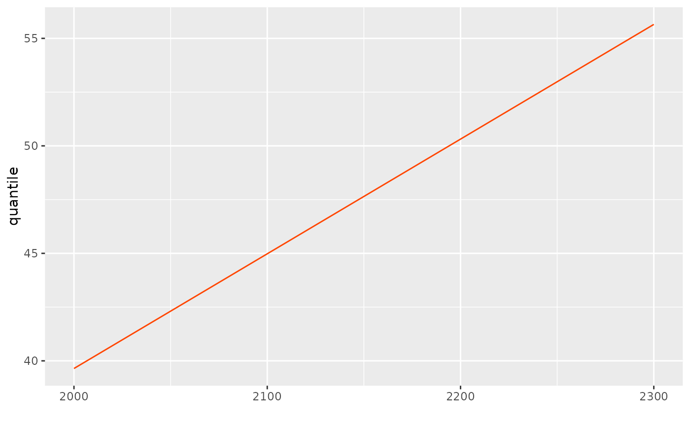
q <- quantile(res2, prob = 1.0 - 1.0 / 200, date = nd)
autoplot(q)

mean(q[1:200])
#> [1] 44.95267