Return Levels and Confidence Intervals for a Poisson-GP Model

Compute return levels along with confidence bounds for a Poisson-GP model with ML inference results.

Usage

# S3 method for poisGP
RL(object, period = NULL, level = 0.70,
   confintMethod = c("proflik", "delta", "none"),
   out = c("data.frame", "array"),
   trace = 0,
   check = FALSE, nCheck = 50, nSigma = 4,
   ftol_abs = 1e-12, ftol_rel = 1e-9,
   ...)

Arguments

object: An object with class "poisGP" representing the inference results for a Poisson-GP model.
period: A vector of periods for which the return levels will be computed. By default "round" periods covering the range from 1 to 1000 are chosen.
level: Level of confidence. Can be a vector.
confintMethod: The method used to compute the confidence intervals. The value "proflik" corresponds to the profile-likelihood. The value "delta" corresponds to the delta method and the value "none" can be used to obtain the return levels without confidence limits on them.
out: The type of outpout wanted, see the Value section.
trace: Integer level of verbosity. The default value is 0, but when confintMethod is "proflik", it is a good practice to use trace = 1, so this may change in the future.
check: Logical If. FALSE the results are intended to be used for a return-level plot, while the value TRUE produce results for a graphical check of the computations.
nCheck: Number of points on a profile-likelihood curve for each value \(T\) of the return period when check is TRUE. These points are taken in an interval containing the ML estimate \(\hat{\rho}(T)\) of the return level \(\rho(T)\), with a range controled by nSigma.
nSigma: Range the of the return levels used to build the curve when check is TRUE. Vector of length two with its values \(n_1\) and \(n_2\) defining the range for the values of \(\rho(T)\) from \(\hat{\rho}(T) - n_1 s(T)\) to \(\hat{\rho}(T) + n_2 s(T)\) where \(s(T)\) is the estimated standard deviation for \(\hat{\rho}(T)\). The default choice usually covers the profile-likelihood interval for all periods. A vector of length one is recycled.
ftol_abs, ftol_rel: Absolute and relative tolerance to stop the constrained optimisation nloptr. These apply to the objective of the constrained optimisation, which is here the return level as a function of the Poisson-GP parameter vector. The smallest possible values reaching convergence should be chosen. By increasing either of thes values the convergence will be easier to get but the results may not be as precise as wanted. This can/should be checked by using check = TRUE and a subsequent call to autoplot.
...: Not used yet.

Value

When check is FALSE (default), an object of class "RL.poisGP" inheriting either from data.frame. It can also be a simple array containing the results. In the first case, the object can be used with the autoplot method to produce the return level plot without recomputing the results.

When check is TRUE the result is an object with class RLCheck.poisGP and can be used with autoplot

to build a graphical check of the results of the profile-likelihood method. This is a list containing two data frames: RL contains the confidence limits and estimates, while negLogLik contains a grid of values for the the return level \(\rho(T)\) along with the corresponding values of the profile negative log-likelihood. This allows to plot the curve.

Details

The return-level curve corresponding to the column or to the dimension named "Quant" is obtained by plugging the ML estimate of the Poisson-GP parameters in the quantile. The confidence limits can be obtained by profile-likelihood or by the standard 'delta' method.

Note

The check for check = TRUE is built by computing the value of the profile-likelihood for each period \(T\) and each candidate value of \(\rho(T)\). This is done by using a two-parameter optimisation: maximise on the vector \([\lambda, \, \xi]\) of the Poisson rate \(\lambda\) and the and GP shape \(\xi\), the return level \(\rho(T)\) being fixed. This optimisation can fail to converge, in which case the result is NA. For now a derivative-free optimisation is used (COBYLA): the computations can be quite long.

Author

Yves Deville

Examples

## ================================================================
## Use the 'Garonne' data from Renext, which embeds both OT data
## and MAX data
## ================================================================
fitp <- poisGP(data = Garonne, threshold = 2900, trace = 2)
#> 
#> The data will not be scaled
#> 
#> Initial values for the parameter
#>      lambda       scale       shape 
#>    1.676923 1026.816514    0.000000 
#> initial  value 927.813009 
#> final  value 925.980426 
#> converged
#> Optimisation results
#> $cvg
#> [1] TRUE
#> 
#> $lb
#> lambda  scale  shape 
#>    0.0    0.0   -0.9 
#> 
#> $ub
#> lambda  scale  shape 
#>    Inf    Inf    Inf 
#> 
#> $df
#> [1] 3
#> 
#> $fit
#> $fit$par
#>        scale        shape 
#> 1287.2134428   -0.1650405 
#> 
#> $fit$value
#> [1] 925.9804
#> 
#> $fit$counts
#> function gradient 
#>       18        6 
#> 
#> $fit$convergence
#> [1] 0
#> 
#> $fit$message
#> NULL
#> 
#> 
#> $estimate
#>        scale        shape 
#> 1287.2134428   -0.1650405 
#> 
#> $negLogLik
#> [1] 925.9804
#> 

## ================================================================
## RL plot with profile-likelihood confidence levels
## ================================================================
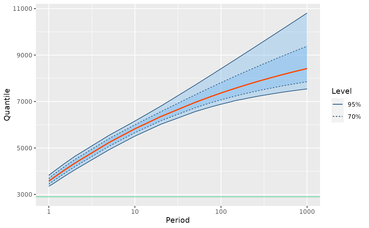
RL <- RL(fitp, out = "data", level = c(0.70, 0.95))
autoplot(RL)


if (FALSE) {
   ## ================================================================
   ## CHECK the results. Quite slow!
   ## ================================================================
   RLc <- RL(fitp, out = "data", level = c(0.70, 0.95),
             check = TRUE)
   autoplot(RLc) + ylim(c(NA, 540)) +
       ggtitle("negative profile log-likelihood for rho(T)")

   ## ================================================================
   ## Using values for ftol_abs or ftol_rel that are not small enough
   ## we get problems in the precision of the result.
   ## ================================================================

   RLc <- RL(fitp, out = "data", level = c(0.70, 0.95), ftol_rel = 1e-5,
             check = TRUE)
   autoplot(RLc) + ylim(c(NA, 540)) +
       ggtitle(paste("negative profile log-likelihood for rho(T) ",
                     " with 'ftol_rel' too large"))
}