Compute Quantiles for the Maximum the Marks of a Poisson-GP Model

The Poisson-GP model given in x only describes the tail of the distribution of the maximum. So when a probability is too small the quantile may be NA.

Usage

# S3 method for pgpTList
quantile(x, newdata = NULL, prob = NULL, level = 0.95, ...)

Arguments

x: An object with class "predict.pgpTList" as created by applying the predict method on an object with class "pgpTList".
newdata: A "new" data frame or Date vector used to define the "new" period. The quantiles will be the those of the random maximum \(M\) of the marks on this period.
prob: Vector of probabilities.
level: The confidence level.
...: Not used yet.

Value

A data frame with columns Prob and Quant.

Details

The computation of the quantiles without any inference result can be performed at a lower cost by using the results of a predict step it these have already been computed. Of course the "new" period will be that which was used in the predict step and can not be changed.

Caution

This method is planned to be renamed as quantMax, to make a clearer difference with the marginal quantiles. The quantMax.pgpTList should thus be used.

Examples

RqU <- rqTList(dailyMet = Rennes, tau = c(0.94, 0.95, 0.96, 0.97, 0.98, 0.99))
Pgp1 <- pgpTList(dailyMet = Rennes, thresholds = RqU, declust = TRUE,
                 fitLambda = TRUE, logLambda.fun = ~YearNum - 1)
#> o Using meteorological variable : "TX"
#> o Adding new variables 
#> o Using K = 3 and the following phases
#> sinjPhi1 sinjPhi2 sinjPhi3 
#>   105.94     8.53    84.21 
#> o Sampling rate : 365.26/year
#> o Looping on 6 thresholds
#> 
#> o Fit the temporal Poisson process:  non-homogeneous
#> 
#> Number of observations  not used in the estimation process:  0
#> Total number of time observations:  28366
#> Number of events:  772
#> 
#> Convergence code:  0
#> Convergence attained
#> Loglikelihood:  -3537.078
#> 
#> Estimated coefficients: 
#>     b0     b1 
#> -3.757  0.009 
#> Full coefficients: 
#>     b0     b1 
#> -3.757  0.009 
#> attr(,"TypeCoeff")
#> [1] "Fixed: No  fixed parameters"
#> 
#> 
#> o Fit the temporal Poisson process:  non-homogeneous
#> 
#> Number of observations  not used in the estimation process:  0
#> Total number of time observations:  28366
#> Number of events:  671
#> 
#> Convergence code:  0
#> Convergence attained
#> Loglikelihood:  -3165.859
#> 
#> Estimated coefficients: 
#>     b0     b1 
#> -3.912  0.010 
#> Full coefficients: 
#>     b0     b1 
#> -3.912  0.010 
#> attr(,"TypeCoeff")
#> [1] "Fixed: No  fixed parameters"
#> 
#> 
#> o Fit the temporal Poisson process:  non-homogeneous
#> 
#> Number of observations  not used in the estimation process:  0
#> Total number of time observations:  28366
#> Number of events:  565
#> 
#> Convergence code:  0
#> Convergence attained
#> Loglikelihood:  -2762.467
#> 
#> Estimated coefficients: 
#>     b0     b1 
#> -4.087  0.010 
#> Full coefficients: 
#>     b0     b1 
#> -4.087  0.010 
#> attr(,"TypeCoeff")
#> [1] "Fixed: No  fixed parameters"
#> 
#> 
#> o Fit the temporal Poisson process:  non-homogeneous
#> 
#> Number of observations  not used in the estimation process:  0
#> Total number of time observations:  28366
#> Number of events:  450
#> 
#> Convergence code:  0
#> Convergence attained
#> Loglikelihood:  -2299.813
#> 
#> Estimated coefficients: 
#>     b0     b1 
#> -4.337  0.012 
#> Full coefficients: 
#>     b0     b1 
#> -4.337  0.012 
#> attr(,"TypeCoeff")
#> [1] "Fixed: No  fixed parameters"
#> 
#> 
#> o Fit the temporal Poisson process:  non-homogeneous
#> 
#> Number of observations  not used in the estimation process:  0
#> Total number of time observations:  28366
#> Number of events:  323
#> 
#> Convergence code:  0
#> Convergence attained
#> Loglikelihood:  -1749.224
#> 
#> Estimated coefficients: 
#>     b0     b1 
#> -4.754  0.016 
#> Full coefficients: 
#>     b0     b1 
#> -4.754  0.016 
#> attr(,"TypeCoeff")
#> [1] "Fixed: No  fixed parameters"
#> 
#> 
#> o Fit the temporal Poisson process:  non-homogeneous
#> 
#> Number of observations  not used in the estimation process:  0
#> Total number of time observations:  28366
#> Number of events:  179
#> 
#> Convergence code:  0
#> Convergence attained
#> Loglikelihood:  -1072.212
#> 
#> Estimated coefficients: 
#>     b0     b1 
#> -5.389  0.018 
#> Full coefficients: 
#>     b0     b1 
#> -5.389  0.018 
#> attr(,"TypeCoeff")
#> [1] "Fixed: No  fixed parameters"
#> 
Date <- seq(from = as.Date("2020-01-01"), to = as.Date("2050-01-01"), by = "day")
## compute the quantile for the maximum on the "new" period
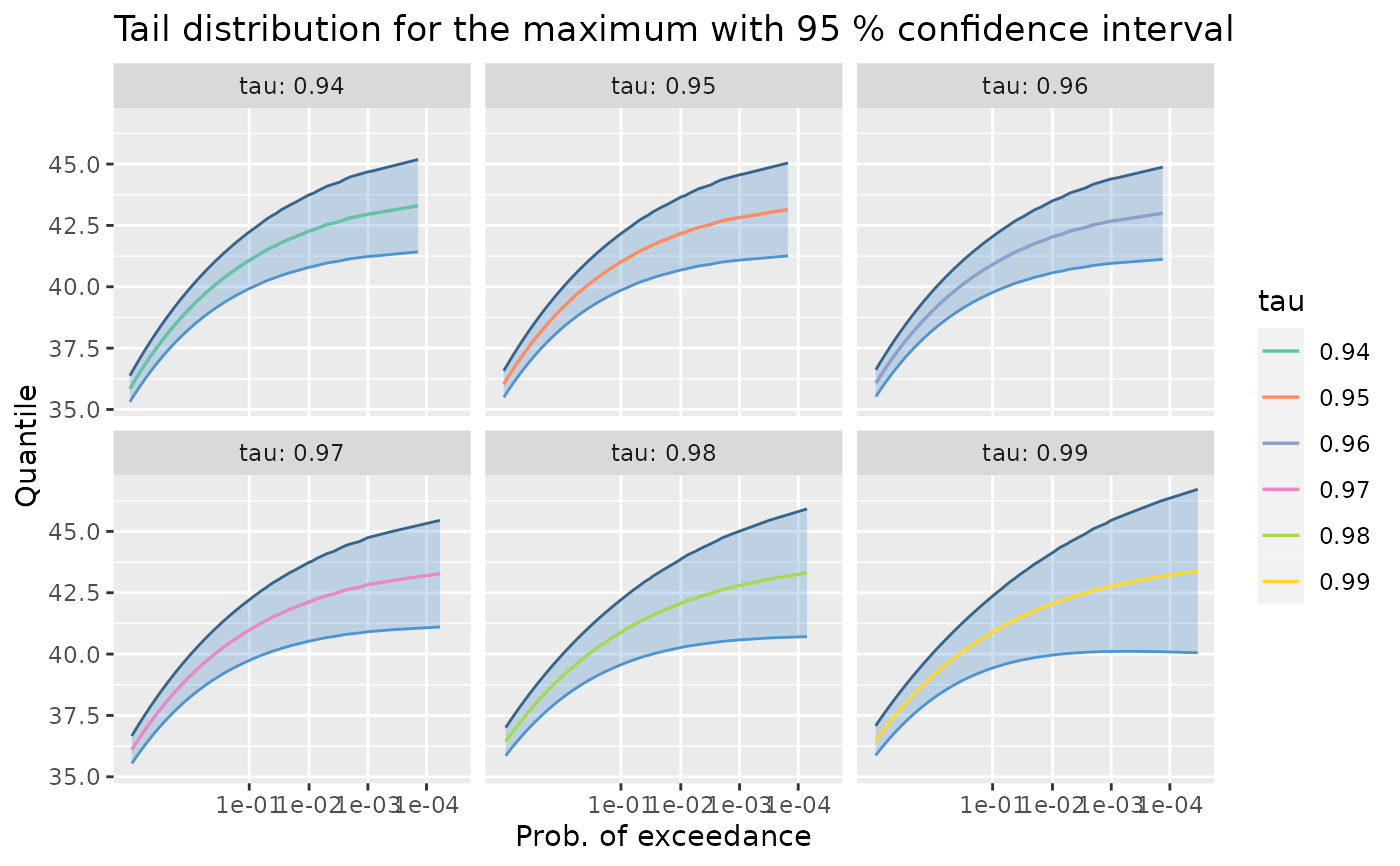
qMax <- quantile(Pgp1, newdata = Date)
autoplot(qMax)