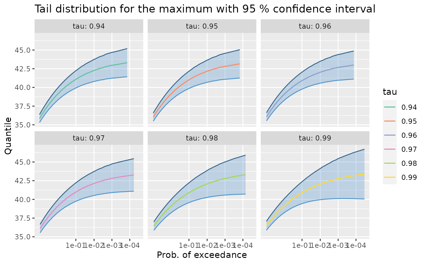
Compute Quantiles for the Maximum the Marks of a Poisson-GP Model

The Poisson-GP model given in x only describes the tail of the distribution of the maximum. So when a probability is too small the quantile may be NA.

Usage

# S3 method for pgpTList
quantMax(object, newdata = NULL, prob = NULL, level = 0.95, ...)

Arguments

object: An object with class "predict.pgpTList" as created by applying the predict method on an object with class "pgpTList".
newdata: A "new" data frame or Date vector used to define the "new" period. The quantiles will be the those of the random maximum \(M\) of the marks on this period.
prob: Vector of probabilities.
level: The confidence level.
...: Not used yet.

Value

A data frame with columns Prob and Quant.

Details

The computation of the quantiles without any inference result can be performed at a lower cost by using the results of a predict step it these have already been computed. Of course the "new" period will be that which was used in the predict step and can not be changed.

Examples

RqU <- rqTList(dailyMet = Rennes, tau = c(0.94, 0.95, 0.96, 0.97, 0.98, 0.99))
Pgp1 <- pgpTList(dailyMet = Rennes, thresholds = RqU, declust = TRUE,
                 fitLambda = TRUE, logLambda.fun = ~YearNum - 1)
#> o Using meteorological variable : "TX"
#> o Adding new variables 
#> o Using K = 3 and the following phases
#> sinjPhi1 sinjPhi2 sinjPhi3 
#>   105.94     8.53    84.21 
#> o Sampling rate : 365.26/year
#> o Looping on 6 thresholds
#> 
#> o Fit the temporal Poisson process:  non-homogeneous
#> 
#> Number of observations  not used in the estimation process:  0
#> Total number of time observations:  28366
#> Number of events:  772
#> 
#> Convergence code:  0
#> Convergence attained
#> Loglikelihood:  -3537.078
#> 
#> Estimated coefficients: 
#>     b0     b1 
#> -3.757  0.009 
#> Full coefficients: 
#>     b0     b1 
#> -3.757  0.009 
#> attr(,"TypeCoeff")
#> [1] "Fixed: No  fixed parameters"
#> 
#> 
#> o Fit the temporal Poisson process:  non-homogeneous
#> 
#> Number of observations  not used in the estimation process:  0
#> Total number of time observations:  28366
#> Number of events:  671
#> 
#> Convergence code:  0
#> Convergence attained
#> Loglikelihood:  -3165.859
#> 
#> Estimated coefficients: 
#>     b0     b1 
#> -3.912  0.010 
#> Full coefficients: 
#>     b0     b1 
#> -3.912  0.010 
#> attr(,"TypeCoeff")
#> [1] "Fixed: No  fixed parameters"
#> 
#> 
#> o Fit the temporal Poisson process:  non-homogeneous
#> 
#> Number of observations  not used in the estimation process:  0
#> Total number of time observations:  28366
#> Number of events:  565
#> 
#> Convergence code:  0
#> Convergence attained
#> Loglikelihood:  -2762.467
#> 
#> Estimated coefficients: 
#>     b0     b1 
#> -4.087  0.010 
#> Full coefficients: 
#>     b0     b1 
#> -4.087  0.010 
#> attr(,"TypeCoeff")
#> [1] "Fixed: No  fixed parameters"
#> 
#> 
#> o Fit the temporal Poisson process:  non-homogeneous
#> 
#> Number of observations  not used in the estimation process:  0
#> Total number of time observations:  28366
#> Number of events:  450
#> 
#> Convergence code:  0
#> Convergence attained
#> Loglikelihood:  -2299.813
#> 
#> Estimated coefficients: 
#>     b0     b1 
#> -4.337  0.012 
#> Full coefficients: 
#>     b0     b1 
#> -4.337  0.012 
#> attr(,"TypeCoeff")
#> [1] "Fixed: No  fixed parameters"
#> 
#> 
#> o Fit the temporal Poisson process:  non-homogeneous
#> 
#> Number of observations  not used in the estimation process:  0
#> Total number of time observations:  28366
#> Number of events:  323
#> 
#> Convergence code:  0
#> Convergence attained
#> Loglikelihood:  -1749.224
#> 
#> Estimated coefficients: 
#>     b0     b1 
#> -4.754  0.016 
#> Full coefficients: 
#>     b0     b1 
#> -4.754  0.016 
#> attr(,"TypeCoeff")
#> [1] "Fixed: No  fixed parameters"
#> 
#> 
#> o Fit the temporal Poisson process:  non-homogeneous
#> 
#> Number of observations  not used in the estimation process:  0
#> Total number of time observations:  28366
#> Number of events:  179
#> 
#> Convergence code:  0
#> Convergence attained
#> Loglikelihood:  -1072.212
#> 
#> Estimated coefficients: 
#>     b0     b1 
#> -5.389  0.018 
#> Full coefficients: 
#>     b0     b1 
#> -5.389  0.018 
#> attr(,"TypeCoeff")
#> [1] "Fixed: No  fixed parameters"
#> 
Date <- seq(from = as.Date("2020-01-01"), to = as.Date("2050-01-01"), by = "day")
## compute the quantile for the maximum on the "new" period
qMax <- quantMax(Pgp1, newdata = Date)
autoplot(qMax)