R Package `dailymet`: Overview

Yves Deville deville.yves@alpestat.com

2023-12-28

Goals

• Use daily meteorological timeseries, mainly TX.

• Provide bases of functions of the date: trigonometric, polynomial, …

• Fit time-varying and non-stationary POT models with emphasis on the sensitivity to the threshold choice, thanks to dedicated classes of objects that we may call “TLists” for list by threshold.

Data classes and data manipulation functions

The "dailyMet" data class

As its name may suggest the "dailyMet" S3 class contains objects describing meteorological timeseries sampled on a daily basis. The package comes with the Rennes example.

library(dailymet)
Rennes

## o Daily Meteorological Time Series
##    o Station:            "Rennes-Saint-Jacques"
##    o Id:                 "07130"
##    o Variable name:      "TX"
##    o Period length (yrs)  77.66
## 
##    o Non-missing periods
##        Start        End Duration
## 1 1945-01-02 2022-08-31    77.66
## 
##    o Summary for variable  TX 
##    Min. 1st Qu.  Median    Mean 3rd Qu.    Max. 
##   -7.50   11.30   15.90   16.18   21.10   40.50 
## 
##    o Five smallest/largest obs
##      min                 max                
## [1,]   -7.5 [1987-01-12]   40.5 [2022-07-18]
## [2,]   -7.0 [1963-01-19]   40.1 [2019-07-23]
## [3,]   -6.6 [1985-01-16]   39.5 [2003-08-05]
## [4,]   -6.3 [1987-01-13]   38.8 [2003-08-09]
## [5,]   -5.9 [1987-01-18]   38.4 [1949-07-12]

The print method used for Rennes shows the summary above which provides the essential information.

class(Rennes)

## [1] "dailyMet"   "data.frame"

methods(class = "dailyMet")

## [1] autoplot head     print    subset   summary  tail    
## see '?methods' for accessing help and source code

So Rennes has class "dailyMet" which inherits from the "data.frame"class. The print method provides useful information. A method which is not implemented for the class "dailyMet" will be inherited from the "data.frame" class e.g., head, tail, nrow …

autoplot(Rennes)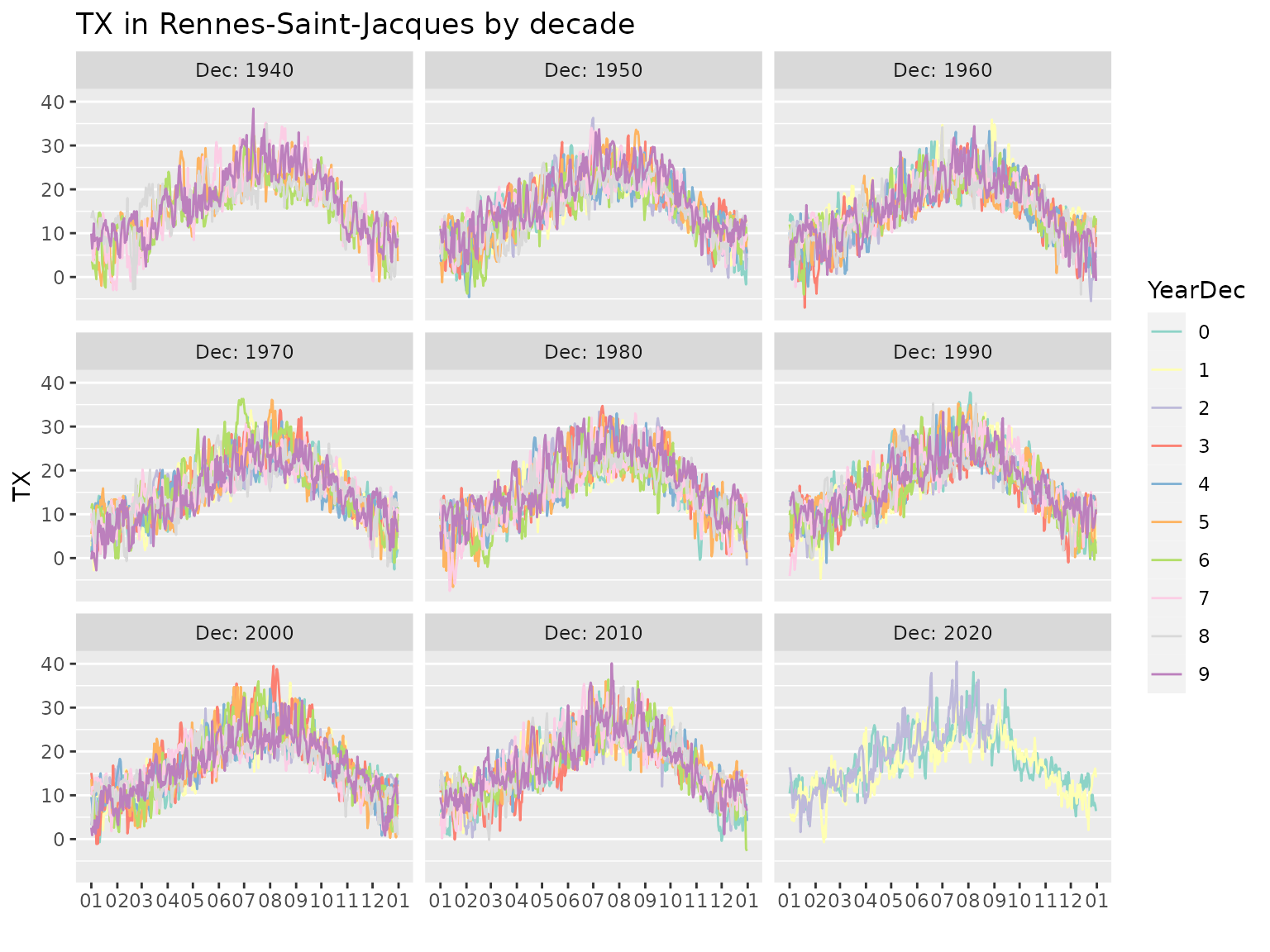

Since the object embeds several variables related to the date, we can use these straightforwardly. Mind that the variable names are capitalised.

autoplot(Rennes, subset = Year >= 2010 & JJA, group = "year")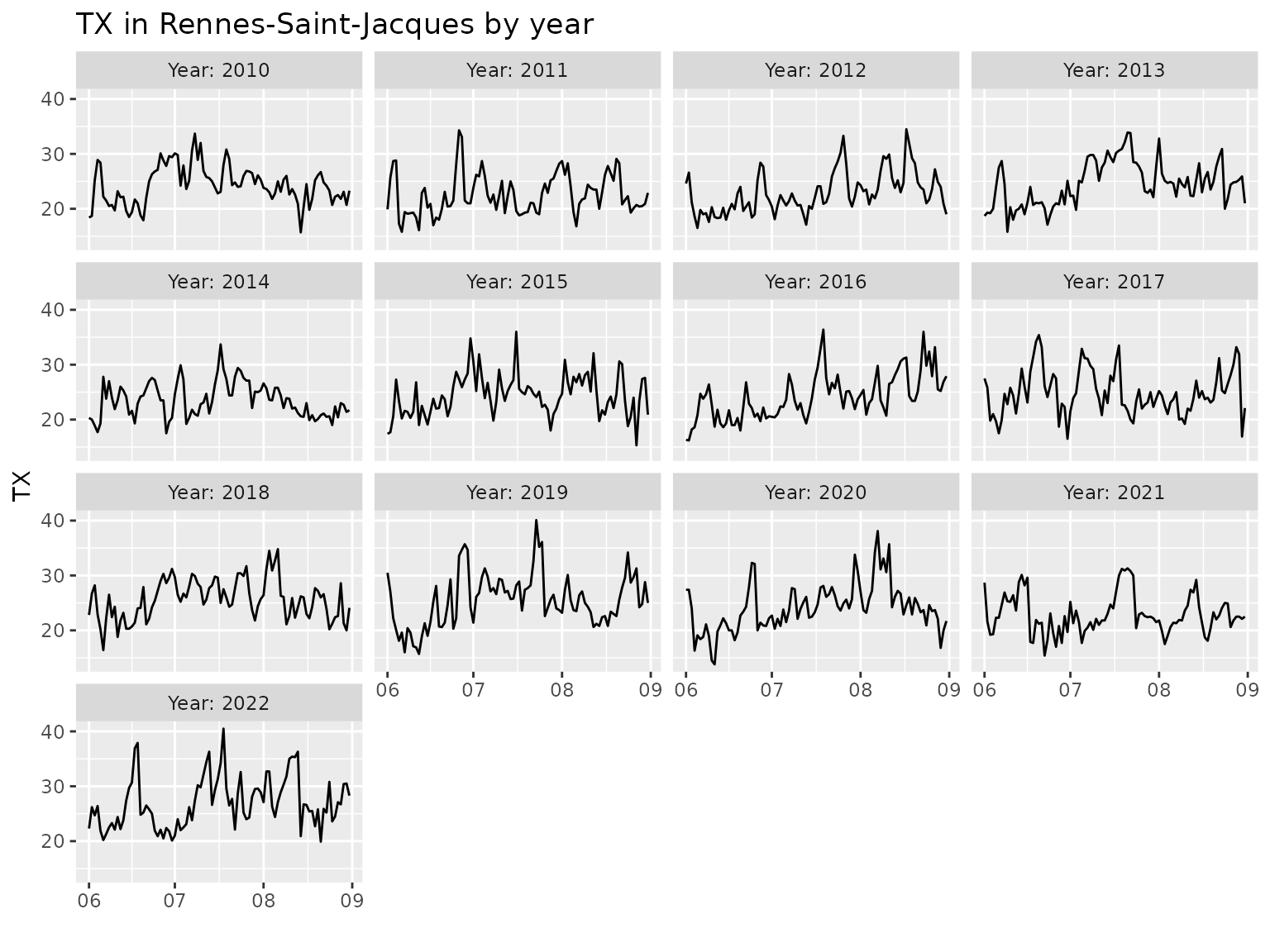

Splitting the timeseries in years is suitable when the interest is on the summer season. It the interest is instead on winter, then using the “winter year” YearW will be better since the whole winter is included in a same “year”.

autoplot(Rennes, subset = Year >= 2010, group = "yearW")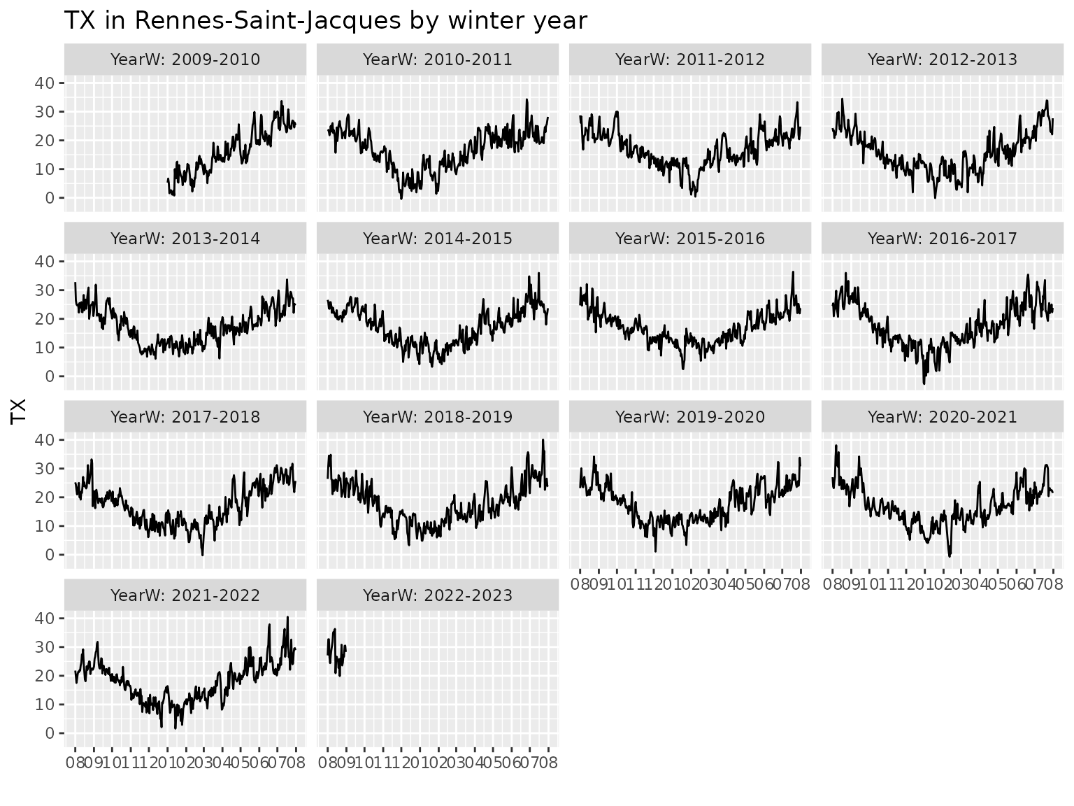

Creating dailyMet objects from data files

Although no other data is shipped with the package, dailymet has a sketch of file-based database, based on the information provided in stationsMF

findStationMF("troy")

##              Desc    Id            Name      Lat  Lon Alt                   Dir
## 1 troyes-barberey 07168 TROYES-BARBEREY 48.32467 4.02 112 07168_troyes-barberey

The idea is that the name or description can be quite loose. The reliable identifier of a station is given in Code, which corresponds to Météo-France données publiques Météo-France

head(stationsMF)

##      Id            Name      Lat       Lon Alt           LongName ShortName
## 1 07005       ABBEVILLE 50.13600  1.834000  69          Abbeville     Abbev
## 2 07015   LILLE-LESQUIN 50.57000  3.097500  47      Lille-Lesquin     Lille
## 3 07020 PTE DE LA HAGUE 49.72517 -1.939833   6 Pointe de la Hague  La-Hague
## 4 07027  CAEN-CARPIQUET 49.18000 -0.456167  67     Caen-Carpiquet      Caen
## 5 07037      ROUEN-BOOS 49.38300  1.181667 151         Rouen-Boos     Rouen
## 6 07072    REIMS-PRUNAY 49.20967  4.155333  95       Reims-Prunay     Reims
##             Zone            Desc OldCode Resol40 Clim
## 1          Somme       abbeville   abbev       1   NW
## 2           Nord   lille-lesquin               1    C
## 3         Manche cap-de-la-hague               1   NW
## 4       Calvados  caen-carpiquet    caen       1   NW
## 5 Seine-Maritime      rouen-boos   rouen       1    C
## 6          Marne    reims-prunay   reims       1    C

We will focus on the French metropolitan area.

See the help stationsMF for a leaflet map of these. Note that the codes of the main MF stations for the metropolitan area correspond roughly to an ordering from North to South (decreasing latitude) and West to East (increasing longitude). This can be of some help.

Provided that the data is available in .csv files suitably named, we can read these into dailyMet objects. The function readMet can be used for that aim. In order to avoid a tedious construction of filenames an automated naming is used. For instance the full information for MF station Troyes (actually at the Troyes-Barberey airport) is found in the list returned by findStationMF. This list can be passed as the first argument of the readMet function, which will build the filename from the values of the Id and Name fields. The file is to be found in a directory with its name stored in the environment variable metData.

## fails: several stations match
try(findStationMF("tro"))

## Several matches found:
## 1 troyes-barberey 07168
## 2 serge-frolow-ile-tromelin 61976
## Error in findStationMF("tro") : several stations match. Hint. use 'id ='

myStation <- findStationMF("troyes")
try(readMet(myStation))

## Error in readMet(myStation) : 
##   The `metData` environment variable is not set. Use `Sys.setenv(metData = x)` to set it.

Sys.setenv(metData = "~/Bureau/climatoData")
try(Troyes <- readMet(myStation))

## Error in readMet(myStation) : 
##   The `metData` environment variable does not define an existing directory.

Although the file is not found, we now see the name of the file that is sought for.

Functions and classes for analyses and models

Peaks Over Threshold (POT) models

The package focusses on so-called Poisson-GP POT models for random observations \(y(t)\) where \(t\) denotes a continuous time index. The model involves a time-varying threshold \(u(t)\) and a time-varying Generalized Pareto distribution for the excess \(y(t) - u(t)\) as recorded at an exceedance time \(y(t) > u(t)\). The exceedance times are assumed to occur according to a Non-Homogeneous Poisson Process (NHPPP) with rate \(\lambda(t)\). The excesses \(y(t) - u(t)\) at the exceedances are asumed to follow the two-parameter Generalised Pareto (GP) distribution with scale \(\sigma(t)>0\) and shape \(\xi(t)\). This distribution has support \((0, \,\infty)\) and the value of the survival function is given for \(x >0\) by \[ S_{\texttt{GP2}}(x;\,\sigma,\,\xi) = \begin{cases} \left[1 + \xi \, x/\sigma \right]_+^{-1/\xi} & \xi \neq 0\\ \exp\{- x/ \sigma \} & \xi = 0 \end{cases} \] where \(z_+:= \max\{z,\, 0\}\) denotes the positive part or a real number \(z\).

In practice, we will consider daily discrete-time timeseries \(y_t\) where \(t\) denotes the day i.e., the date. Similarly, the threshold \(u_t\), the rate \(\lambda_t\) and the GP parameters \(\sigma_t\) and \(\xi_t\) will be daily non random) timeseries. Provided that the exceedance rate is small enough, a discrete-time framework can be deduced from the continuous-time one. This model can also be related as well to the Binomial-GP model where the daily exceedance probabillity is small enough.

Using TLists

What are TLists?

A T-list or is a list of objects sharing the same definition except for their threshold. The threshold is related to a probability tau corresponding to the probability \(\tau\) as used in quantile regression.

• A rqTList object is a list of rq objects differing only by their probability tau, hence related to the same data, same formula, …

• A fevdTList object is a list of fevd objects representing Poisson-GP POT models differing only by their threshold which is given by quantile regression and corresponds to different probabilities tau. Again the fevdobjects are related to the same data, to the same formulas, …

Implicitly assumed, the vector tau should be in strictly increasing order.

Another TList class is the "pgpTList" class which corresponds to a list of fitted Poisson-GP models. Mind that consistently with rq and fevd a lower case acronym is used, followed by "TList“. However, for now, the class "pgp" does not exist. We can fit a pgpTList object with a vector tau of length one, if needed. A pgpTList object is quite similar to a fevdList object. The main difference concerns the exceedances and their occurrence in time: Instead of an assuming constant rate \(\lambda\), a purely temporal non-homogeneous Poisson process is used. A rate depending on the time \(\lambda(t)\) or on the time and other covariates \(\lambda(\mathbf{x})\) can be specified by using a devoted formula for \(\log \lambda\).

Caution The development of pgpTList class and of the relevant methods is far from being achieved. Some major changes are likely to occur. For now the methods are as follows.

methods(class = "pgpTList")

##  [1] exceed        logLik        makeNewData   modelMatrices parInfo      
##  [6] predict       print         quantile      quantMax      residuals    
## [11] simulate      summary      
## see '?methods' for accessing help and source code

Some important remarks

• A rq object does not encode a full distribution nor even a tail distribution. The rq objects may fail to be consistent and the quantile may fail to increase with the probability \(\tau\). See (Northrop, Jonathan, and Randell 2016).

• Strictly speaking, the fevd objects in a fevdTList object are different Poisson-GP models, although they must have the same formulas. Indeed, the Poisson-GP parameterisation is not independent of the threshold: if the GPD scale depends linearly of a covariate \(x\) for a given threshold \(u\), then for a higher threshold \(u'>u\) the scale will generally depend on \(x\) in a nonlinear fashion. See the relation between the two POT parameterisation Poisson-GP and NHPP, only the later being independent of the threshold.

Quantile regression for seasonality

Rq <- rqTList(dailyMet = Rennes)
tau(Rq)

## tau=0.50 tau=0.70 tau=0.80 tau=0.90 tau=0.95 tau=0.97 tau=0.98 tau=0.99 
##     0.50     0.70     0.80     0.90     0.95     0.97     0.98     0.99

formula(Rq)

## TX ~ Cst + cosj1 + sinj1 + cosj2 + sinj2 + cosj3 + sinj3 - 1
## NULL

autoplot(Rq)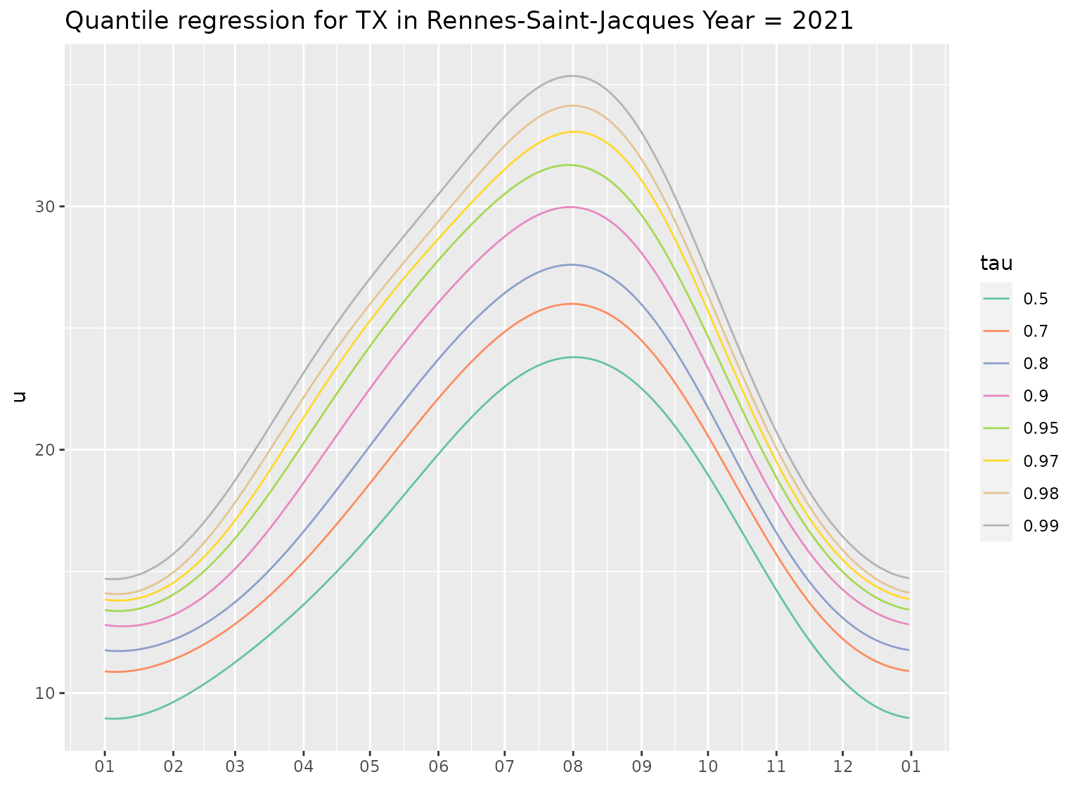

By default the creator rqTList

• Uses some defined probabilities \(\tau\) for the quantiles. These can be assessed by the tau method.

• Uses a formula which defines a yearly seasonality for the quantiles. The default formula uses a basis of trigonometric functions with 3 harmonics, corresponding the the fundamental frequency \(1/365.25\:\text{day}^{-1}\) and its integer multiples \(2/365.25\), \(3/365.25\), …

• Considers a “design” function which creates the required variables cosj1 , sinj1, cosj2, sinj2, … where the integer after the prefix cos of sin gives the frequency in increasing order, standing for the fundamental frequency corresponding to the one-year period.

• Build the required variables from the existing variables in the object specified by dailyMet, mainly from the Date column.

• Fits quantile regression rq objects from the quantreg package

More precisely the quantile \(q(\tau)\) of the meteorological variable is considered as a trigonometric polynomial function \(q_d(\tau)\) of the day in the year \(d\) (\(1 \leqslant d \leqslant 366\))

\[\begin{equation} \tag{1} q_d(\tau) \approx \alpha_0^{q}(\tau) + \sum_{k=1}^K \alpha_k^{q}(\tau) \cos\{2\pi k d/D\} + \beta_k^{q}(\tau) \sin\{2\pi k d/D\} \end{equation}\]

where \(D:=365.25\) is yearly period expressed in days. The pseudo-exponent \(q\) in the coefficients \(\alpha\) and \(\beta\) is used to recall that they describe a quantile. The default number of harmonics \(K\) is \(3\). The quantile regression provides the estimated coefficients \(\hat{\alpha}_k^{q}(\tau)\) and \(\hat{\beta}_k^{q}(\tau)\).

methods(class = "rqTList")

##  [1] autolayer autoplot  coef      coSd      formula   predict   print    
##  [8] summary   tau       xi       
## see '?methods' for accessing help and source code

coef(Rq)

##               Cst     cosj1     sinj1       cosj2     sinj2       cosj3
## tau=0.50 16.06393 -6.799077 -2.591552 -0.25845982 0.8639527 -0.03092440
## tau=0.70 17.95239 -7.088085 -2.512324 -0.05437666 0.8490012  0.09359081
## tau=0.80 19.16725 -7.533421 -2.492802 -0.04192276 0.8351121  0.17707189
## tau=0.90 20.91793 -8.261868 -2.391511 -0.10477575 0.8021272  0.26742011
## tau=0.95 22.24216 -8.813697 -2.265968 -0.24878473 0.8232536  0.24753280
## tau=0.97 23.12972 -9.185094 -2.350450 -0.41137561 0.9621417  0.32897144
## tau=0.98 23.81042 -9.465539 -2.349878 -0.47458855 1.0689253  0.25157101
## tau=0.99 24.73573 -9.763231 -2.296899 -0.50022134 1.1528784  0.24505818
##                sinj3
## tau=0.50  0.06418181
## tau=0.70  0.06247610
## tau=0.80  0.04022597
## tau=0.90 -0.05661638
## tau=0.95 -0.09498655
## tau=0.97 -0.17853494
## tau=0.98 -0.26641707
## tau=0.99 -0.27323854

coSd(Rq)

##          Cst            cosj1          sinj1          cosj2         
## tau=0.50 16.064 [0.027] -6.799 [0.042] -2.592 [0.034] -0.258 [0.037]
## tau=0.70 17.952 [0.029] -7.088 [0.042] -2.512 [0.040] -0.054 [0.041]
## tau=0.80 19.167 [0.035] -7.533 [0.052] -2.493 [0.047] -0.042 [0.049]
## tau=0.90 20.918 [0.039] -8.262 [0.053] -2.392 [0.056] -0.105 [0.054]
## tau=0.95 22.242 [0.048] -8.814 [0.066] -2.266 [0.069] -0.249 [0.067]
## tau=0.97 23.130 [0.061] -9.185 [0.084] -2.350 [0.088] -0.411 [0.086]
## tau=0.98 23.810 [0.065] -9.466 [0.086] -2.350 [0.098] -0.475 [0.090]
## tau=0.99 24.736 [0.081] -9.763 [0.120] -2.297 [0.110] -0.500 [0.115]
##          sinj2          cosj3          sinj3         
## tau=0.50  0.864 [0.037] -0.031 [0.037]  0.064 [0.037]
## tau=0.70  0.849 [0.041]  0.094 [0.040]  0.062 [0.040]
## tau=0.80  0.835 [0.049]  0.177 [0.046]  0.040 [0.046]
## tau=0.90  0.802 [0.054]  0.267 [0.051] -0.057 [0.051]
## tau=0.95  0.823 [0.067]  0.248 [0.063] -0.095 [0.063]
## tau=0.97  0.962 [0.085]  0.329 [0.080] -0.179 [0.080]
## tau=0.98  1.069 [0.089]  0.252 [0.085] -0.266 [0.084]
## tau=0.99  1.153 [0.115]  0.245 [0.108] -0.273 [0.108]

The coSd method (for “coef” and “Standard error” or “Standard deviation”) gives the coefficients and their standard error. We see that some estimated coefficients are not significant, namely those for the 3-rd harmonic for the “small” probabilities. However, when \(\tau\) becomes larger, the estimated coefficients for the \(3\)-rd harmonic becomes significant, although their standard error increases because they are based on a smaller number of observations. This suggests that the \(3\)-rd harmonic plays a role in the seasonality of the extremes, although it will be difficult to assess.

As may be guessed from the plot of quantiles, the fitted phases corresponding to the different harmonics are quite similar across probabilities \(\tau < 0.95\). More precisely we may consider the following alternative parameterisation of the trigonometric polynomial

\[\begin{equation} \tag{2} q_d(\tau) \approx \gamma_0^{q}(\tau) + \sum_{k=1}^K \gamma_k^{q}(\tau) \sin\left\{2\pi k \left[d - \phi_k^{q}(\tau)\right]/D\right\} \end{equation}\]

where the parameter \(\gamma_k^{q}(\tau)\) and \(\phi_k^{q}(\tau)\) are called amplitudes and phase shifts or simply phases. The two formulations (1) and (2) are actually equivalent, as can be seen from the trigonometric “angle subtraction formula” \(\sin(a -b) = \sin(a)\cos(b) - \cos(a) \sin(b)\). We could think of using the second form in a quanteg::rq fit, but this is not possible since the phase \(\phi_k^q\) appears in a nonlinear fashion. So we can fit the linear cos-sin form and then compute the estimate for the amplitudes and phases by using some trigonometry.

co <- coef(Rq)
phases(co)

##          phi1  phi2  phi3 gamma1 gamma2 gamma3
## tau=0.50  112  8.45   8.7   7.28  0.902 0.0712
## tau=0.70  111  1.86 -19.0   7.52  0.851 0.1125
## tau=0.80  110  1.46 -26.1   7.94  0.836 0.1816
## tau=0.90  108  3.78  87.3   8.60  0.809 0.2733
## tau=0.95  106  8.53  84.2   9.10  0.860 0.2651
## tau=0.97  106 11.74  81.7   9.48  1.046 0.3743
## tau=0.98  105 12.14  75.5   9.75  1.170 0.3664
## tau=0.99  105 11.90  75.0  10.03  1.257 0.3670

The table shows the \(K=3\) phases \(\phi_k\) and amplitudes \(\gamma_k\). Note that the object returned by phases has as special class "phasesMatrix". The amplitudes are actually stored as an attribute of the numeric matrix of phases, not as a matrix with \(2K\) columns.

We see that for the different probabilities the phases of the \(1\)-st and \(2\)-nd harmonics are quite similar, while those of the \(3\)-rd harmonics are different, and seem to drift as the probability \(\tau\) increases.

autoplot(phases(co))

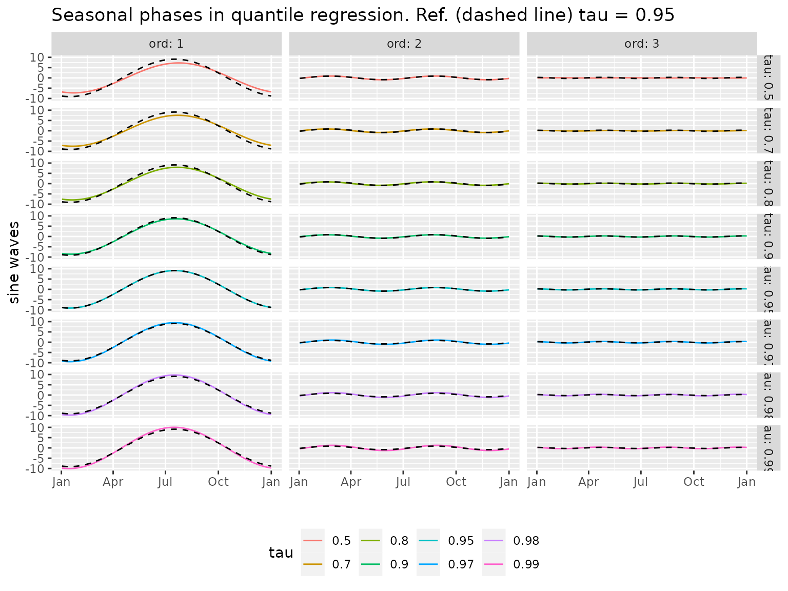
The constant \(\gamma_0^{[\tau]}\) does not appear on the plot.. Note that the amplitudes \(\gamma_k^{[\tau]}\) rapidly decrease with the frequency, consistently with the fact that the quantiles are quite smooth functions of the day \(d\). The amplitude slightly increases with \(\tau\), especially for the fundamental frequency \(k=1\). In other words the seasonality becomes more pronounced when the probability \(\tau\) increases.

Seasonality in (time-varying) POT models

Why seasonality matters

Using a suitable description of the seasonality is a major concern in POT modelling (Coles and Tawn 2005), (Coles 2004), (Northrop, Jonathan, and Randell 2016). Concerning our meteorological variables, a natural idea is to use GP or GEV parameters depending on the date through the day in year \(d\) since it is clear that the marginal distribution heavily depends on \(d\).

There are also many reasons to use a seasonally time-varying threshold \(u(d)\) depending as well on \(d\). One motivation is the efficiency of the estimation: A constant threshold would be too low for a season and too high for another. Moreover, if a constant threshold is used, the results are likely to depend much on the threshold value because the distribution over a period of several months in the year is actually a weighted mixture of different distributions corresponding to the values of \(d\), and their weight will depend much on the constant threshold. For instance, if a constant threshold is used for all the JJA period, the weight of the early June and late August will be smaller when the threshold is increased.

Seasonal Poisson-GP models

In order to describe the yearly seasonality, a natural idea is to use a trigonometric polynomial as described above. For instance the GP scale parameter \(\sigma\) could depend on \(t\) though the day in year \(d\) as in

\[ \sigma_d = \alpha_0^{\sigma} + \sum_{k=1}^K \alpha_k^{\sigma} \cos\{2\pi k d/D\} + \beta_k^{\sigma} \sin\{2\pi k d/D\} \]

where the coefficients \(\alpha_k^{\sigma}\) and \(\beta_k^{\sigma}\) are to be estimated. However \(2 K +1\) parameters and for \(K=3\) or even for \(K=2\) the estimation can be difficult. To facilitate the estimation, one can use instead the amplitude-phase formulation

\[ \sigma_d = \gamma_0^{\sigma} + \sum_{k=1}^K \gamma_k^{\sigma} \sin\left\{2\pi k \left[d - \phi_k \right]/D\right\} \]

where the phases \(\phi_k\) are considered as fixed or known. In practice, we can use the phases \(\phi_k := {\hat{\phi}}^{q}_k(\tau_{\text{ref}})\) given by quantile regression for a fixed “reference” probability e.g., \(\tau_{\text{ref}} = 0.95\). So we have only \(K+1\) parameter to estimate. Since the phases are usually quite stable for the high quantiles, hopefully the same should be true also for the GP parameters.

The "fevdTlist" is a transitional class which requires to “manually” create a list of fevd objects having the same but different thresholds obtained by quantile regression. Once these objects have been fitted and gathered in a list, the as.fevdTList coercion method can be used. The "pgpTList" class is easier to use.

Note that while using as above a large range of probability \(\tau\) is adequate to get insights on the variable, a narrower range of probability values seems more adequate for POT models. We can use \(\tau\) ranging, say, from \(0.90\) to \(0.98\).

To create a pgpTList object, the appropriate way is first, fit a rqTList object with chosen thresholds. This object will be passed to the thresholds argument of the creator pgpTList. In order to compute the sine wave basis functions with the prescribed phases corresponding to the probability \(\tau_{\text{ref}}\), the argument tauRef can be used.

Rq <- rqTList(dailyMet = Rennes, tau = c(0.94, 0.95, 0.96, 0.97, 0.98, 0.99))
Pgp1 <- pgpTList(dailyMet = Rennes, thresholds = Rq,
                declust = TRUE, fitLambda = TRUE, logLambda.fun = ~ YearNum - 1)
pred <- predict(Pgp1, lastFullYear = TRUE)
autoplot(pred, facet = FALSE)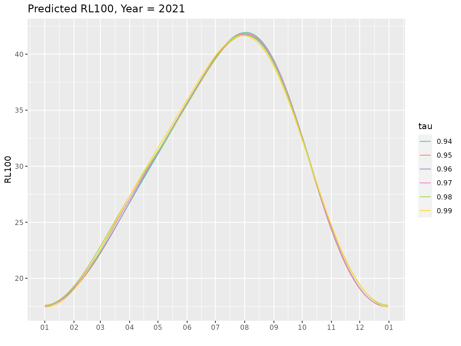

The output of the code was not shown because the NHPoisson::fitPP.fun function used to fit the time part of the model is very verbose. The Figure above shows the 100-year return level (RL), which depends on the date, for the last full year of the fitting period. We see that rather realistic values are obtained and moreover that the fitted RL depends little on the threshold choice, which is a nice feature. The default formulas used in the creator for the GP part (hence passed to fevd) are

• scale.fun = ~Cst + sinjPhi1 + sinJPhi2 + sinjPhi3 - 1

• shape.fun = ~1

So no time-trend was specified in the GP part of the model. However a time-trend was used for the exceedance rate, namely \[ \lambda(t) = \exp\{ \beta_0^\lambda + \beta_1^\lambda t \}, \] where the time \(t\) is given by YearNum so the coefficient \(\beta^\lambda_1\) is in inverse years \(\text{yr}^{-1}\).

How pgpTList works

The value of tauRef is used to select the appropriate line in the matrix phases(coef(thresholds)) which is used internally. So tauRef must correspond to a probability used to define the thresholds. The so-created vector of phases phi is then used to create the basis functions with the sinBasis function or equivalently of the tsDesign function with type = "sinwave". The sine wave basis functions are used to add new variables to the data frame given in dailyMet. Then the “fitting functions” extRemes::fevd and NHPoisson:fitPP.fun are used to fit the “GP” part” and the (temporal) “Poisson part” for each of the thresholds computed from the thresholds object. The results for the “GP” part and the the time Poisson part are stored as the two elements "GP" and "timePoisson" of the returned list, the first having the class "fevdTList". We hence can use the methods for the "fevdTList" class to get insights on the "GP" part of our pgpTList object.

Caution The log-likelihood of a Poisson-GP is the sum of two contributions corresponding to the GP and the time-Poisson parts, see Northrop et Al.

Phi <- phases(coef(Rq))

Investigating the distribution of the maximum

Goal

One often wants to investigate the distribution of the maximum \(M := \max_t y_t\) where the maximum is taken on a “new” period of interest, typically a period in the near future. By using a Poisson-GP POT model one can only investigate the tail-distribution of \(M\). More precisely the Poisson-GP model allows the computation of \(\text{Pr}\{M \leqslant m\}\) when \(m\) is larger than the maximum of the thresholds on the period of interest \(m> \max_t u(t)\). The reason is that when this condition holds the condition \(M > m\) is equivalent to \(M_{\texttt{peak}} > m\) where \(M_{\texttt{peak}}\) denotes the maximum of the peaks on the same period.

One can show that \[ \log \text{Pr}\{M \leqslant m \} = -\int \lambda_u(t) \, S_{\texttt{GP2}}\{m - u(t);\, \sigma_u(t), \, \xi(t)\}\, \text{d}t, \qquad \text{for } m \text{ large}, \] where the time integral is on the period of interest, and the discrete-time approximation is \[ \log \Pr\{ M \leqslant m \} \approx - \frac{1}{365.25} \, \sum_t \lambda_{u,t} \, S_{\texttt{GP2}}(m - u_t;\, \sigma_t,\, \xi_t), \qquad \text{for } m \text{ large}. \]

In both cases the condition \(m \text{ large}\) is more precisely \(m > \max_t u(t)\) or \(m> \max_t u_t\).

Note that \(M\) does not follow a Generalized Extreme Value (GEV) distribution, even in its tail, but has the same tail as a mixture of GEV distributions. In particular if the shape \(\xi_t\) is chosen to be time-varying then the largest values of \(\xi_t\) will have a disproportionate impact on the high quantiles.

Using the quantile method

The quantile method can be used to compute the tail quantiles from a pgpTList object

Date <- seq(from = as.Date("2020-01-01"),
            to = as.Date("2050-01-01"), by = "day")
qMax <- quantMax(Pgp1, newdata = Date)
autoplot(qMax)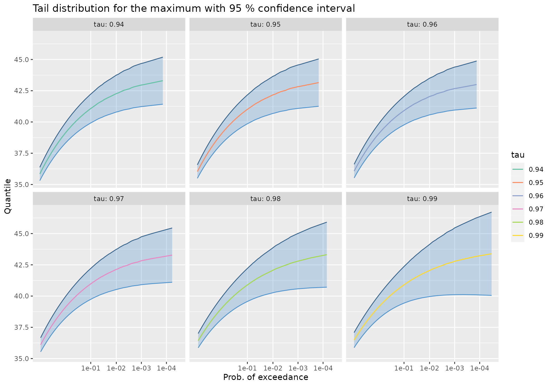

We can display the quantiles in a table

knitr::kable(subset(format(qMax), tau == 0.96))

	tau	Prob	ProbExc	Quant	L	U	Level
93	0.96	0.950	0.050	41.32	40.08	42.57	0.95
97	0.96	0.980	0.020	41.76	40.39	43.14	0.95
99	0.96	0.990	0.010	42.04	40.57	43.50	0.95
102	0.96	0.995	0.005	42.27	40.72	43.82	0.95
103	0.96	0.995	0.005	42.27	40.72	43.82	0.95
106	0.96	0.998	0.002	42.53	40.87	44.18	0.95
107	0.96	0.999	0.001	42.67	40.95	44.40	0.95

Note that the class "pgpTList" has a format method used here. This method rounds the quantiles and confidence limit digits but it also selects “round” exceedance probabilities such as 0.1, 0.01 as is often needed in reports. To save space, only the quantiles corresponding to one value of \(\tau\) are shown here.

Using the simulate method

As an alternative we can simulate the (declustered) exceedances on the period of interest. By default only the large exceedances will be simulated. More precisely, for each value of \(\tau\) a new threshold \(v := \max_{t} u(t)\) is defined and only the exceedances over \(v\) will be considered. These events occur in summer.

sim <- simulate(Pgp1)
autoplot(sim)

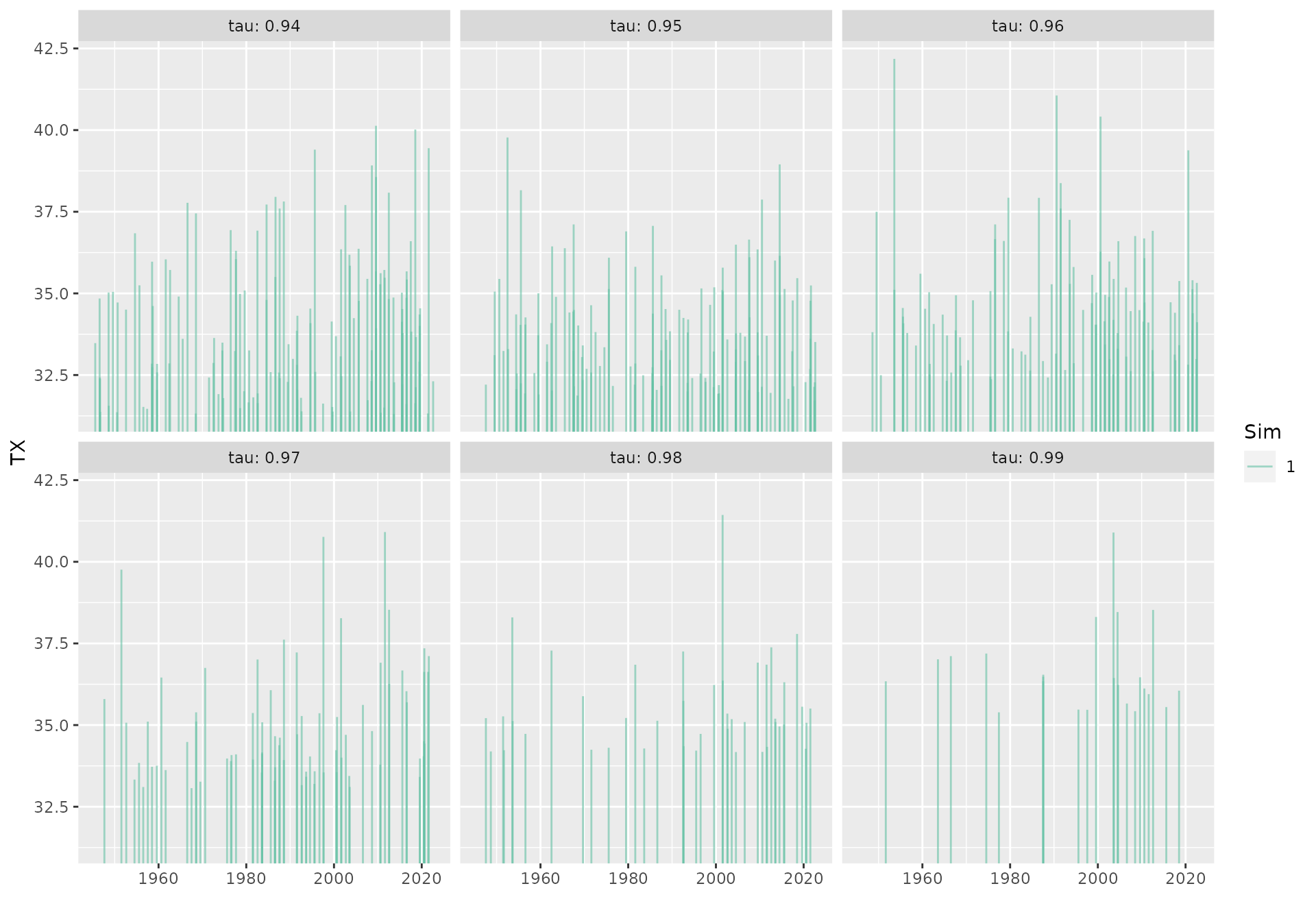
By default, only one simulation is done. But by using the formal argument nsim with a large value (say nsim = 1000 or more) we can compute estimate quantiles, see the help ?simulate.PgpTList. For each simulation \(k=1\), \(\dots\), \(K\) where \(K\) is given by nsim, the simulate method provides the random exceedance times \(T_i^{[k]}\) and the related random marks \(Y_i^{[k]}\) for \(i=1\), \(\dots\), \(N^{[k]}\) where \(N^{[k]}\) is random and varies across simulations. We then have a sample of \(K\) maxima \(M^{[k]} := \max_i Y_i^{[k]}\) and the sample quantiles of the \(M^{[k]}\) should be close to those given by the quantile method.

Mind that a large value of \(K\) used must be chosen large to estimate the quantiles and that the simulate method can be quite slow. Also some warnings are likely to be thrown related to rounding the exceedance times. The explanation is that the simulation of the exceedance times \(T_i\) is based on a continuous-time Poisson Process, so that some rounding is needed to get dates and this can lead “ex-aequo” that must be discarded.

Appendix

Technical issues

Related to quantreg

• An rq object as created by quantreg::rq does not store the data used.

• Coping with missing value NA is difficult because the default prediction corresponds to na.omit which removes the observations with NA response.

Related to extRemes

• An object with class "fevd" corresponding to a Poisson-GP POT model does not fit the “time part” of the process. There is usually no reason to assume that the exceedance rate is constant.

• An object with class "fevd" corresponding to a Poisson-GP POT model does not store the value of the threshold as required to make a prediction on a new data. Consequently the predict method for the "fevd" class as implemented in dailymet is unreliable because an attempt is made to find the threshold from the stored call, but the corresponding objects are most often not found.

Related to NHPoisson

• There is no formula interface for fitPP.fun. The covariates are given in a numeric matrix. The coefficients do not have appealing names and the order of the columns in the matrix of covariates matters.

• The class "mlePP" corresponding to the objects created by fitPP.mle does not have a predict method.

References

Coles, Stuart. 2004. “The Use and Misuse of Extreme Value Models in Practice.” In Extreme Values in Finance, Telecommunications, and the Environment, edited by Bärbel Finkenstädt and Holger Rootzén. Chapman & Hall.

Coles, Stuart, and Jonathan Tawn. 2005. “Seasonal Effects of Extreme Surges.” Stochastic Environmental Research and Risk Assessment 19 (6): 417–27. https://doi.org/10.1007/s00477-005-0008-3.

Northrop, Paul J., Philip Jonathan, and David Randell. 2016. “Threshold Modelling of Non-Stationary Extremes.” In Extreme Value Modeling and Risk Analysis, edited by D. K. Dey and J. Yan. Chapman & Hall.