Fit a non-stationary Poisson-GP Model using several Thresholds computed by Quantile Regression.

Fit a non-stationary Poisson-GP model for several thresholds given in the rqTList object thresholds corresponding to a vector of probability.

Usage

pgpTList(
  dailyMet,
  subset = NULL,
  thresholds,
  declust = TRUE,
  tauRef = 0.95,
  fitLambda = FALSE,
  logLambda.fun = ~1,
  scale.fun = ~Cst + sinjPhi1 + sinjPhi2 + sinjPhi3 - 1,
  shape.fun = ~1,
  extraDesign = NULL,
  trace = 1
)

Arguments

dailyMet: An object with class "dailyMet" containing the data.
subset: A character defining a condition used to subset the data, typically to select a period within the year e.g., summer. Note that the condition is applied after declustering and there are side effects: The exceedances in the first two days or last two days of a period within year may be lost. NOT IMPLEMENTED YET. Note that the condition is used only for the Extreme Value part of the model, not on the determination of the threshold. Therefore, the fitted thresholds remain unchanged whether the the condition is used or not.
thresholds: An object with class "rqTList" containing the thresholds.
declust: Logical. If TRUE the exceedances over each threshold will be declustered.
tauRef: The reference probability defining the quantile regression fit that will be used to define the phases of the sine waves.
fitLambda: Logical. If TRUE the temporal Poisson process is fitted, using the formula logLambda.fun.
logLambda.fun: Formula for the log-rate of the time Poisson process. For now, there are only a few possibilities. See Details. Mind that only numeric covariates can be used.
scale.fun, shape.fun: Formulas for the GP scale and shape as in fevd.
extraDesign: A list with a specific structure used to generate extra "design variables" that can be used in formulas, see Examples and the help of designVars and rqTList for examples of syntax. By default a trigonometric design with three harmonics is used, along with the sinus waves basis corresponding to the phases of the reference threshold defined by tauRef. The sinus wave variables are created by using the sinBasis function with the relevant value of phi.
trace: Integer level of verbosity.

Value

An object with class "pgpTList". This is a list with the following elements

tau The vector of probabilities extracted from thresholds.
thresholds A copy of thresholds as given on entry.
GP A list with class fevdTList
logLambda.fun, scale.fun, scale.fun The formulas used for the "GP part" of the model.

Details

For each probability tau[i]

Find the exceedances over the threshold corresponding to the probability tau[i], and decluster these if wanted.
Fit a non-stationary GP model using extRemes::fevd with type = "GP" and with the formulas prescribed.
Fit a non-stationary temporal Poisson process model using NHPoisson::fitPP.fun.

The formula given in logLambda.fun will typically involve YearNum. Note that the constant is alaways included by the function NHPoisson::fitPP.fun so it should be discarded from the formula when covariates are used. For instance in order to use the covariare YearNum we must use the formla ~ YearNum -1.

Note

The use of subset, still experimental, is aimed to focus the estimation on a period within the year, typically summer or winter. This should not be used to use a shorter timeseries. The rate of the temporal Poisson process is computed on the basis of the full times series, not on the basis of the cumulated duration of the subset. For instance if subset selects 6 months in a year and if the timeseries duration is 60 year, then the rate is still computed on the basis of a 60-year duration, not on a 30-year duration.

Caution

At the time being, a pgpTList object is not a list of pgp objects. The output is likely to be re-designed, so a pgpTList object is better used via methods.

Examples

## define the thresholds with the default seasonality, see 'rqTList'
Rq <- rqTList(dailyMet = Rennes,
              tau = c(0.94, 0.95, 0.96, 0.97, 0.98, 0.99))

## fit
Pgp1 <- pgpTList(dailyMet = Rennes, thresholds = Rq,
                 declust = TRUE,
                 fitLambda = TRUE, logLambda.fun = ~ YearNum - 1)
#> o Using meteorological variable : "TX"
#> o Adding new variables 
#> o Using K = 3 and the following phases
#> sinjPhi1 sinjPhi2 sinjPhi3 
#>   105.94     8.53    84.21 
#> o Sampling rate : 365.26/year
#> o Looping on 6 thresholds
#> 
#> o Fit the temporal Poisson process:  non-homogeneous
#> 
#> Number of observations  not used in the estimation process:  0
#> Total number of time observations:  28366
#> Number of events:  772
#> 
#> Convergence code:  0
#> Convergence attained
#> Loglikelihood:  -3537.078
#> 
#> Estimated coefficients: 
#>     b0     b1 
#> -3.757  0.009 
#> Full coefficients: 
#>     b0     b1 
#> -3.757  0.009 
#> attr(,"TypeCoeff")
#> [1] "Fixed: No  fixed parameters"
#> 
#> 
#> o Fit the temporal Poisson process:  non-homogeneous
#> 
#> Number of observations  not used in the estimation process:  0
#> Total number of time observations:  28366
#> Number of events:  671
#> 
#> Convergence code:  0
#> Convergence attained
#> Loglikelihood:  -3165.859
#> 
#> Estimated coefficients: 
#>     b0     b1 
#> -3.912  0.010 
#> Full coefficients: 
#>     b0     b1 
#> -3.912  0.010 
#> attr(,"TypeCoeff")
#> [1] "Fixed: No  fixed parameters"
#> 
#> 
#> o Fit the temporal Poisson process:  non-homogeneous
#> 
#> Number of observations  not used in the estimation process:  0
#> Total number of time observations:  28366
#> Number of events:  565
#> 
#> Convergence code:  0
#> Convergence attained
#> Loglikelihood:  -2762.467
#> 
#> Estimated coefficients: 
#>     b0     b1 
#> -4.087  0.010 
#> Full coefficients: 
#>     b0     b1 
#> -4.087  0.010 
#> attr(,"TypeCoeff")
#> [1] "Fixed: No  fixed parameters"
#> 
#> 
#> o Fit the temporal Poisson process:  non-homogeneous
#> 
#> Number of observations  not used in the estimation process:  0
#> Total number of time observations:  28366
#> Number of events:  450
#> 
#> Convergence code:  0
#> Convergence attained
#> Loglikelihood:  -2299.813
#> 
#> Estimated coefficients: 
#>     b0     b1 
#> -4.337  0.012 
#> Full coefficients: 
#>     b0     b1 
#> -4.337  0.012 
#> attr(,"TypeCoeff")
#> [1] "Fixed: No  fixed parameters"
#> 
#> 
#> o Fit the temporal Poisson process:  non-homogeneous
#> 
#> Number of observations  not used in the estimation process:  0
#> Total number of time observations:  28366
#> Number of events:  323
#> 
#> Convergence code:  0
#> Convergence attained
#> Loglikelihood:  -1749.224
#> 
#> Estimated coefficients: 
#>     b0     b1 
#> -4.754  0.016 
#> Full coefficients: 
#>     b0     b1 
#> -4.754  0.016 
#> attr(,"TypeCoeff")
#> [1] "Fixed: No  fixed parameters"
#> 
#> 
#> o Fit the temporal Poisson process:  non-homogeneous
#> 
#> Number of observations  not used in the estimation process:  0
#> Total number of time observations:  28366
#> Number of events:  179
#> 
#> Convergence code:  0
#> Convergence attained
#> Loglikelihood:  -1072.212
#> 
#> Estimated coefficients: 
#>     b0     b1 
#> -5.389  0.018 
#> Full coefficients: 
#>     b0     b1 
#> -5.389  0.018 
#> attr(,"TypeCoeff")
#> [1] "Fixed: No  fixed parameters"
#> 

## try a varying GP shape 'xi'
if (FALSE) {
    Pgp2 <- pgpTList(dailyMet = Rennes, thresholds = Rq,
                     declust = TRUE, 
                     shape.fun = ~ Cst + sinjPhi1 + sinjPhi2 + sinjPhi3 - 1,
                     fitLambda = TRUE, logLambda.fun = ~ YearNum - 1)
}
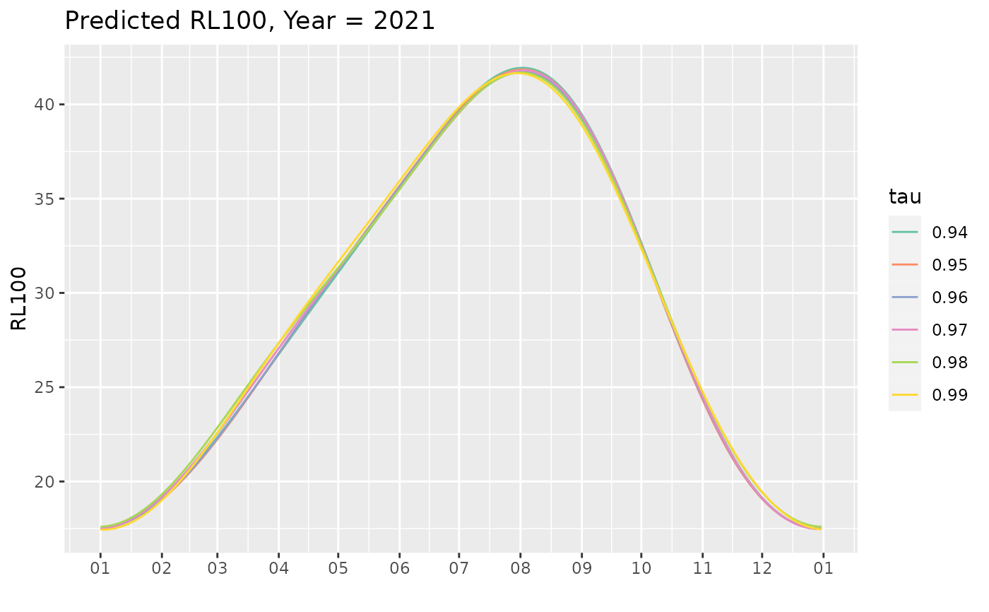
## plot one year to 
predYear <- predict(Pgp1, last = TRUE)
gYear <- autoplot(predYear, facet = FALSE)
gYear


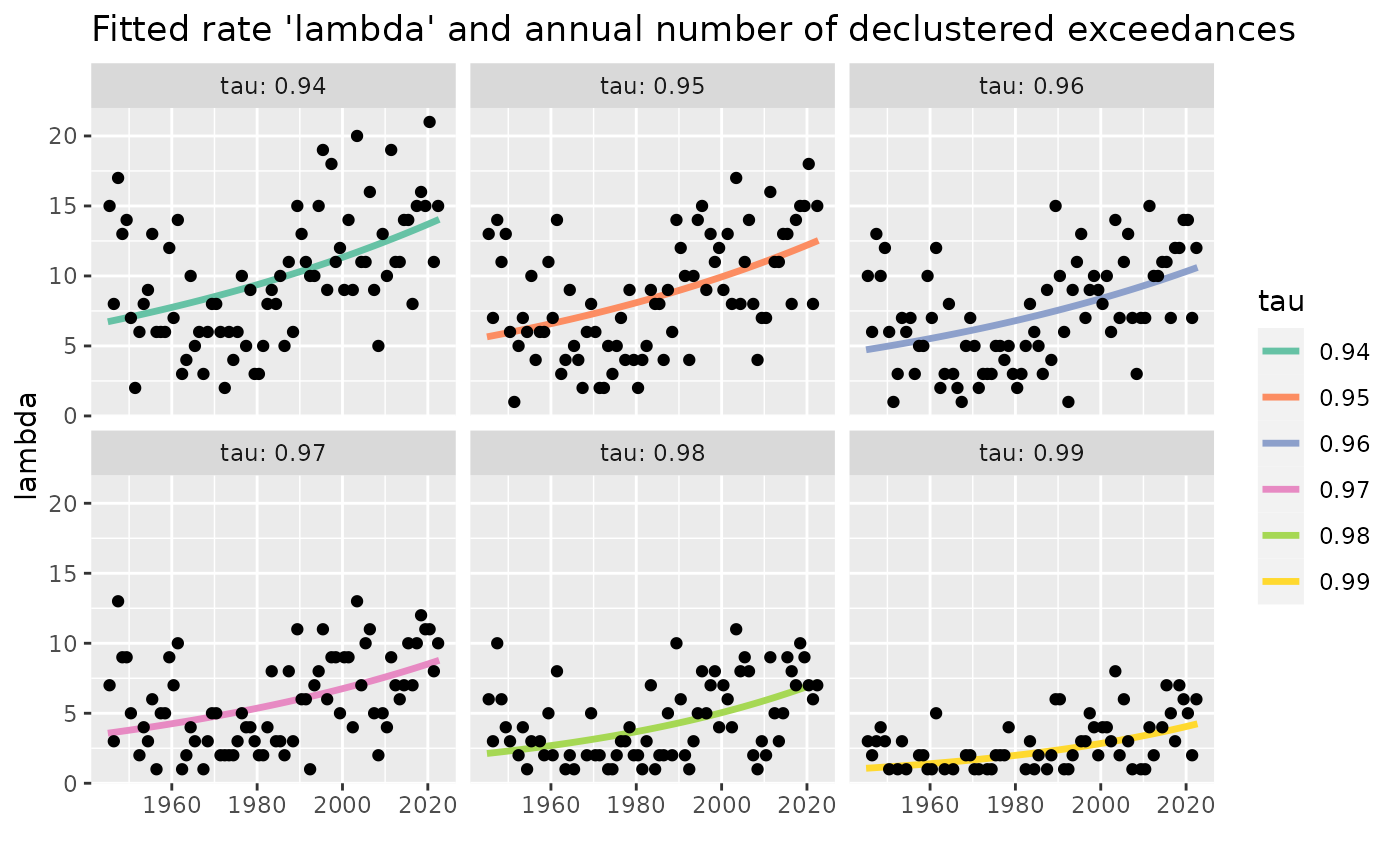
## show the evolution of the exceedance rate on the long-run
predAll <- predict(Pgp1, last = FALSE)
exceed <- exceed(Pgp1)
gAll <- autoplot(predAll, which = "lambda", size = 1.2) +
            geom_point(data = exceed, mapping = aes(x = Date, y = Nb)) +
                ggtitle(paste("Fitted rate 'lambda' and annual number of",
                              "declustered exceedances"))
gAll


## Add an extra design corresponding to broken line splines. This
## creates a new variable 't1_1970' that can be used in formula to
## assess a possible change in the trend at the beginning of the seventies.
Pgp3 <-
    pgpTList(dailyMet = Rennes, thresholds = Rq,
             declust = TRUE,
             fitLambda = TRUE,
             logLambda.fun = ~ YearNum + t1_1970 - 1,
             extraDesign =
                 list("breaks" = list(what = "NSGEV::breaksX",
                                      args = list(breaks = "1970-01-01"))))
#> o Using meteorological variable : "TX"
#> o Adding new variables 
#> o Using K = 3 and the following phases
#> sinjPhi1 sinjPhi2 sinjPhi3 
#>   105.94     8.53    84.21 
#>    o evaluation of `NSGEV::breaksX`. Date is added in 1-st arg `date`
#> o Sampling rate : 365.26/year
#> o Looping on 6 thresholds
#> 
#> o Fit the temporal Poisson process:  non-homogeneous
#> 
#> Number of observations  not used in the estimation process:  0
#> Total number of time observations:  28366
#> Number of events:  772
#> 
#> Convergence code:  0
#> Convergence attained
#> Loglikelihood:  -3521.467
#> 
#> Estimated coefficients: 
#>     b0     b1     b2 
#> -4.108 -0.026  0.046 
#> Full coefficients: 
#>     b0     b1     b2 
#> -4.108 -0.026  0.046 
#> attr(,"TypeCoeff")
#> [1] "Fixed: No  fixed parameters"
#> 
#> 
#> o Fit the temporal Poisson process:  non-homogeneous
#> 
#> Number of observations  not used in the estimation process:  0
#> Total number of time observations:  28366
#> Number of events:  671
#> 
#> Convergence code:  0
#> Convergence attained
#> Loglikelihood:  -3151.093
#> 
#> Estimated coefficients: 
#>     b0     b1     b2 
#> -4.280 -0.027  0.049 
#> Full coefficients: 
#>     b0     b1     b2 
#> -4.280 -0.027  0.049 
#> attr(,"TypeCoeff")
#> [1] "Fixed: No  fixed parameters"
#> 
#> 
#> o Fit the temporal Poisson process:  non-homogeneous
#> 
#> Number of observations  not used in the estimation process:  0
#> Total number of time observations:  28366
#> Number of events:  565
#> 
#> Convergence code:  0
#> Convergence attained
#> Loglikelihood:  -2746.698
#> 
#> Estimated coefficients: 
#>     b0     b1     b2 
#> -4.505 -0.032  0.055 
#> Full coefficients: 
#>     b0     b1     b2 
#> -4.505 -0.032  0.055 
#> attr(,"TypeCoeff")
#> [1] "Fixed: No  fixed parameters"
#> 
#> 
#> o Fit the temporal Poisson process:  non-homogeneous
#> 
#> Number of observations  not used in the estimation process:  0
#> Total number of time observations:  28366
#> Number of events:  450
#> 
#> Convergence code:  0
#> Convergence attained
#> Loglikelihood:  -2286.767
#> 
#> Estimated coefficients: 
#>     b0     b1     b2 
#> -4.765 -0.032  0.056 
#> Full coefficients: 
#>     b0     b1     b2 
#> -4.765 -0.032  0.056 
#> attr(,"TypeCoeff")
#> [1] "Fixed: No  fixed parameters"
#> 
#> 
#> o Fit the temporal Poisson process:  non-homogeneous
#> 
#> Number of observations  not used in the estimation process:  0
#> Total number of time observations:  28366
#> Number of events:  323
#> 
#> Convergence code:  0
#> Convergence attained
#> Loglikelihood:  -1738.267
#> 
#> Estimated coefficients: 
#>     b0     b1     b2 
#> -5.223 -0.034  0.063 
#> Full coefficients: 
#>     b0     b1     b2 
#> -5.223 -0.034  0.063 
#> attr(,"TypeCoeff")
#> [1] "Fixed: No  fixed parameters"
#> 
#> 
#> o Fit the temporal Poisson process:  non-homogeneous
#> 
#> Number of observations  not used in the estimation process:  0
#> Total number of time observations:  28366
#> Number of events:  179
#> 
#> Convergence code:  0
#> Convergence attained
#> Loglikelihood:  -1066.829
#> 
#> Estimated coefficients: 
#>    b0    b1    b2 
#> -5.83 -0.03  0.06 
#> Full coefficients: 
#>    b0    b1    b2 
#> -5.83 -0.03  0.06 
#> attr(,"TypeCoeff")
#> [1] "Fixed: No  fixed parameters"
#> 
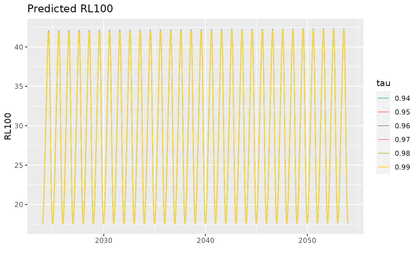
p3 <- predict(Pgp3,
              newdata = data.frame(Date = seq(from = as.Date("2024-01-01"),
                                   to = as.Date("2054-01-01"),
                                   by = "day")))
autoplot(p3, facet = FALSE)


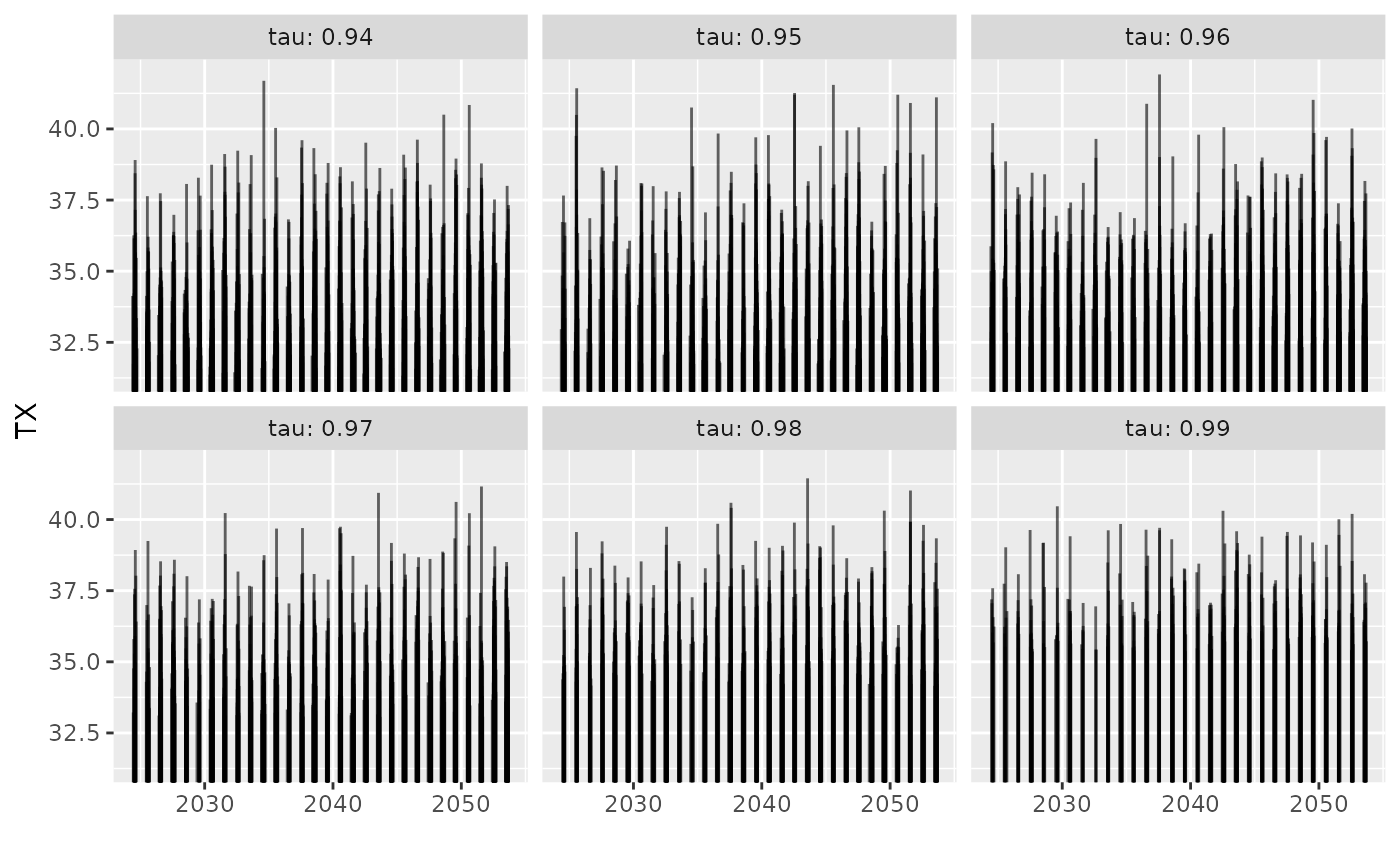
## simulate 
s3 <- simulate(Pgp3, nsim = 10,
              newdata = data.frame(Date = seq(from = as.Date("2024-01-01"),
                                   to = as.Date("2054-01-01"),
                                   by = "day")))
#> Warning: collapsing to unique 'x' values
#> Warning: collapsing to unique 'x' values
#> Warning: collapsing to unique 'x' values
#> Warning: collapsing to unique 'x' values
#> Warning: collapsing to unique 'x' values
#> Warning: collapsing to unique 'x' values
#> Warning: collapsing to unique 'x' values
#> Warning: collapsing to unique 'x' values
#> Warning: collapsing to unique 'x' values
#> Warning: collapsing to unique 'x' values
#> Warning: collapsing to unique 'x' values
#> Warning: collapsing to unique 'x' values
#> Warning: collapsing to unique 'x' values
#> Warning: collapsing to unique 'x' values
#> Warning: collapsing to unique 'x' values
#> Warning: collapsing to unique 'x' values
#> Warning: collapsing to unique 'x' values
#> Warning: collapsing to unique 'x' values
#> Warning: collapsing to unique 'x' values
#> Warning: collapsing to unique 'x' values
#> Warning: collapsing to unique 'x' values
#> Warning: collapsing to unique 'x' values
#> Warning: collapsing to unique 'x' values
#> Warning: collapsing to unique 'x' values
#> Warning: collapsing to unique 'x' values
#> Warning: collapsing to unique 'x' values
#> Warning: collapsing to unique 'x' values
#> Warning: collapsing to unique 'x' values
#> Warning: collapsing to unique 'x' values
#> Warning: collapsing to unique 'x' values
#> Warning: collapsing to unique 'x' values
#> Warning: collapsing to unique 'x' values
#> Warning: collapsing to unique 'x' values
#> Warning: collapsing to unique 'x' values
#> Warning: collapsing to unique 'x' values
#> Warning: collapsing to unique 'x' values
#> Warning: collapsing to unique 'x' values
#> Warning: collapsing to unique 'x' values
#> Warning: collapsing to unique 'x' values
#> Warning: collapsing to unique 'x' values
#> Warning: collapsing to unique 'x' values
#> Warning: collapsing to unique 'x' values
#> Warning: collapsing to unique 'x' values
#> Warning: collapsing to unique 'x' values
#> Warning: collapsing to unique 'x' values
#> Warning: collapsing to unique 'x' values
#> Warning: collapsing to unique 'x' values
#> Warning: collapsing to unique 'x' values
#> Warning: collapsing to unique 'x' values
#> Warning: collapsing to unique 'x' values
#> Warning: collapsing to unique 'x' values
#> Warning: collapsing to unique 'x' values
#> Warning: collapsing to unique 'x' values
#> Warning: collapsing to unique 'x' values
#> Warning: collapsing to unique 'x' values
#> Warning: collapsing to unique 'x' values
#> Warning: collapsing to unique 'x' values
#> Warning: collapsing to unique 'x' values
#> Warning: collapsing to unique 'x' values
#> Warning: collapsing to unique 'x' values
autoplot(s3)