Overview of the beverstan package

Note

This report was generated with knitr::spin. Do not edit Rmarkdown file by hand!

library(beverstan)

Bayes TVGEV for the annual maxima of temperature in Dijon

`TVGEVBayes` objects

The function TVGEVBayes is very similar to NSGEV::TVGEV function. It uses the same arguments: data, Date, response to define the data frame to use and the name of the variables date and response in it. The date variable must be either a column with class "Date" or a column that can be coerced with as.Date, typically a character giving dates in POSIX format. The response contains the annual maxima of daily maximal values (TX) as recorded in Dijon-Longvic (France). The data where provided by the European Climate Assesment & Dataset.

The design argument contains R language: a call to a function returning a design matrix. Then the three formulas loc, scale and shape specify the dependence of the GEV parameters on the date. Here we will use a design for a “regression kink”: the response is a broken line with a change of slope at a threshold point here chosen as 1970.

df <- within(TXMax_Dijon, Date <- as.Date(sprintf("%4d-01-01", Year)))
fit <- TVGEVBayes(data = df,
                  date = "Date", response = "TXMax",
                  design = breaksX(date = Date, breaks = "1970-01-01", degree = 1),
                  loc = ~ t1 + t1_1970, scale = ~ 1, shape = ~ 1,
                  seed = 1234)

## Warning: There were 1 divergent transitions after warmup. See
## https://mc-stan.org/misc/warnings.html#divergent-transitions-after-warmup
## to find out why this is a problem and how to eliminate them.

## Warning: Examine the pairs() plot to diagnose sampling problems

The output of the previous code chunk was not shown. The warning can require further investigation, see later.

class(fit)

## [1] "TVGEVBayes"

methods(class = "TVGEVBayes")

## [1] autoplot coef     fitted   predict  print    profLik  RL       summary 
## [9] vcov    
## see '?methods' for accessing help and source code

So we can use autoplot.

autoplot(fit) + ggtitle("Posterior mean for the GEV expectation") + theme_gray()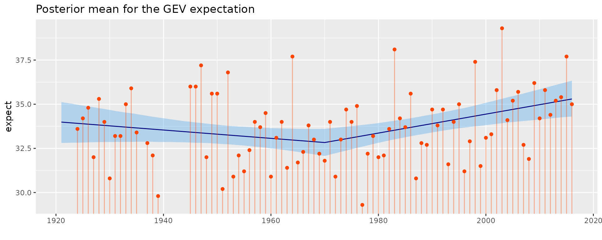

The posterior mean of the GEV expectation is shown along with a $95\%$ credible interval on it. Of course, the credible interval should not be confouded with a prediction interval, which would be much larger.

Instead of the GEV expectation, we can similarly plot a quantile.

autoplot(fit, which = "quantile", prob = 0.95) + theme_gray() +
     ggtitle("Posterior mean for the GEV quantile with probability 0.95")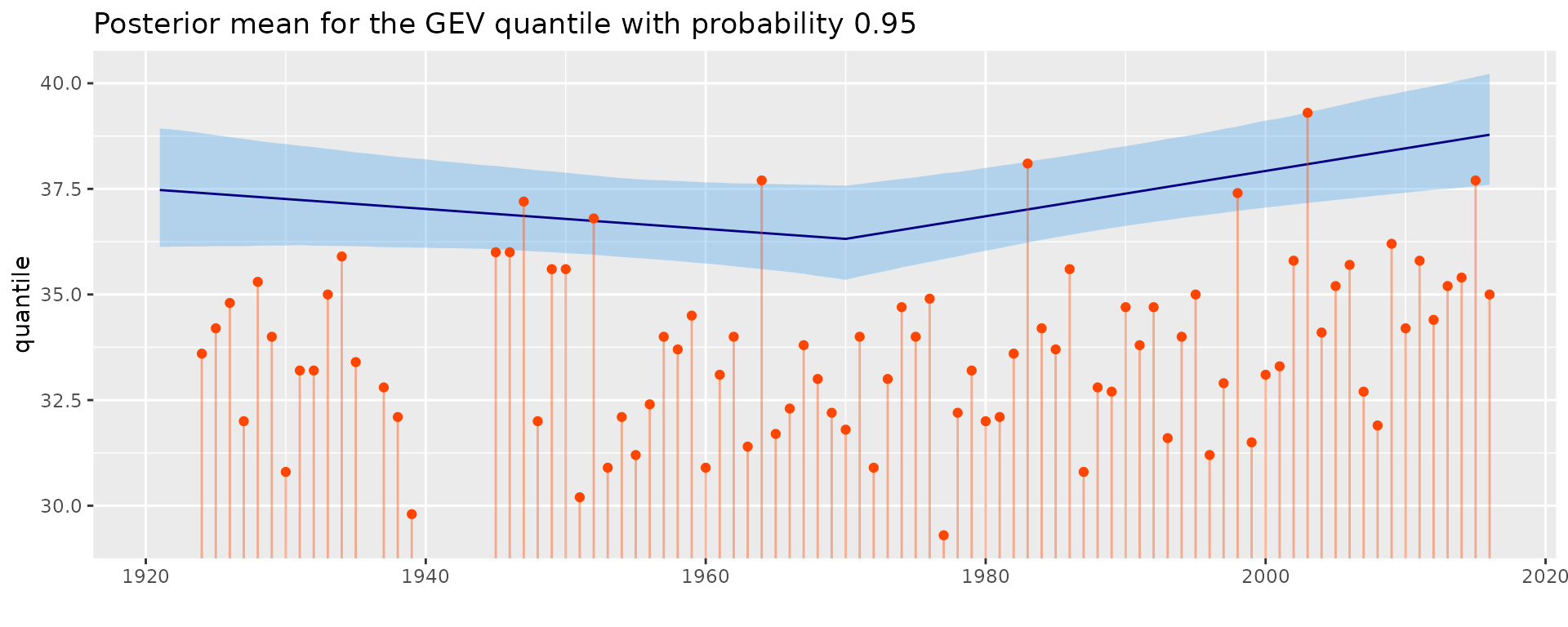

Now try the summary method

summary(fit)

## o Call
## TVGEVBayes(data = df, date = "Date", response = "TXMax", design = breaksX(date = Date, 
##     breaks = "1970-01-01", degree = 1), loc = ~t1 + t1_1970, 
##     scale = ~1, shape = ~1, seed = 1234)
## 
## o Parameters
##                MAP post. mean post. sd post. L post. U
## mu_0       32.0391    32.0418   0.3909 31.2701 32.7965
## mu_t1      -0.0279    -0.0236   0.0164 -0.0546  0.0086
## mu_t1_1970  0.0829     0.0772   0.0288  0.0196  0.1341
## sigma_0     1.7696     1.8273   0.1561  1.5526  2.1666
## xi_0       -0.1930    -0.1706   0.0736 -0.3046 -0.0170

To remind of the design, we can apply the call on the data frame

des <- with(df, breaksX(date = Date,  breaks = "1970-01-01", degree = 1))
des

## Block time series
## 
## o First block: 1921-01-01
## o Last block:  2016-01-01
## 
##       date          t1     t1_1970 
## 1921-01-01 -48.9993155   0.0000000 
## 1922-01-01 -48.0000000   0.0000000 
## 1923-01-01 -47.0006845   0.0000000 
##   ... <more rows>
## 2014-01-01  44.0000000  44.0000000 
## 2015-01-01  44.9993155  44.9993155 
## 2016-01-01  45.9986311  45.9986311

autoplot(des) + ggtitle("Design basis") + theme_gray()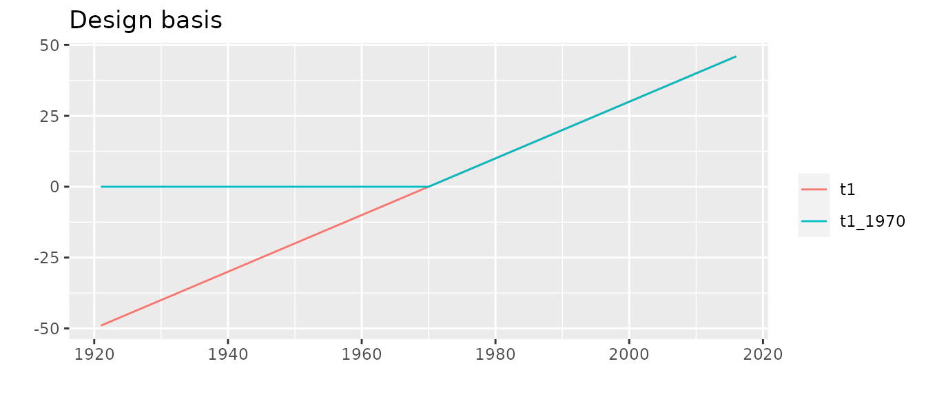

The column "t1" defines a linear trend with a slope of $1~\text{year}^{-1}$ . The colmun "t1_1970" defines a broken line with a change of slope located at year $1970$ : the slopes are $1~\text{year}^{-1}$ before $1970$ , then $1~\text{year}^{-1}$ . The parameter names are automatically build by pasting the GEV parameter name "mu", "sigma" or "xi" with the name of the variable entering the formula. Note however that the constant is not taken as "(Intercept)" as in lm and many other models, but "0". In the present case, the eventual slope (after year 1970) is the sum of mu_t1 and mu_t1_1970 because the two basis functions are non-zero then. So for instance the posterior mean for the eventual slope is 0.0536 $\text{C}/\text{year}^{-1}$ or 0.536 $\text{C}/\text{decade}^{-1}$ .

We can see the (Bayesian) estimates of the parameters, along with $95\%$ credible intervals. Insasmuch the credible interval on mu_t1_1970 does not contain $0$ , we can say that the two slopes before and after $1970$ are significantly different.

We can extract the coefficients with the coef method. Since we may want either the MAP or the posterior mean, the method has an ususual argument type which allows to make a choice.

coef(fit)

##        mu_0       mu_t1  mu_t1_1970     sigma_0        xi_0 
## 32.03912611 -0.02790677  0.08289061  1.76955738 -0.19296432

coef(fit, type = "postMean")

##        mu_0       mu_t1  mu_t1_1970     sigma_0        xi_0 
## 32.04182925 -0.02361283  0.07721219  1.82728067 -0.17062777

As its name may suggest, the RL method Return Level plot.

myRL <- RL(fit)
autoplot(myRL) + theme_gray() + ggtitle("Return level plot")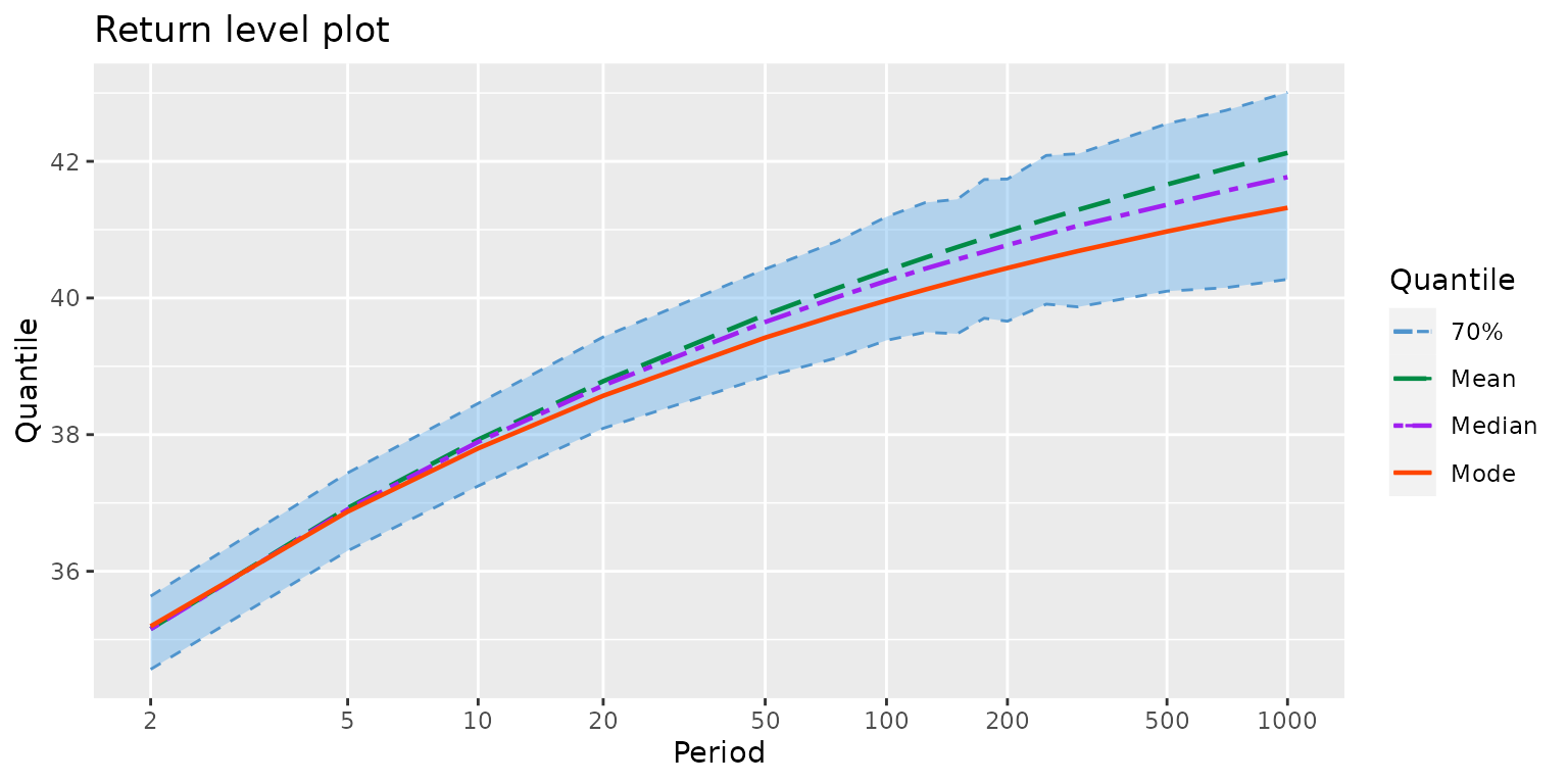

The credible limits are empirical quantiles of the MCMC iterates which explains their wiggling aspect. They can be smoothed, although this is only for aesthetical reasons.

myRL <- RL(fit, smooth = TRUE)
autoplot(myRL) + theme_gray() + ggtitle("Return level plot (smoothed credible limits)")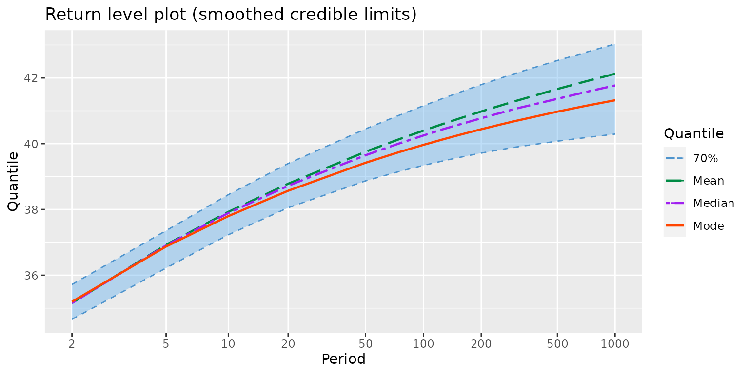

We can use the predict method

myPred <- predict(fit)
tail(myPred)

##    newTimeRange  Prob    Quant
## 15    2016_2017 0.008 40.81713
## 16    2016_2017 0.005 41.29651
## 17    2016_2017 0.004 41.52736
## 18    2016_2017 0.003 41.83012
## 19    2016_2017 0.002 42.27019
## 20    2016_2017 0.001 43.07133

The column newTimeRange indicates the time range (or period) on which the prediction is computed. Note that Prob is the probability of exceedance, so in the classical cas where the extremes are the large value, the interest is mainly on the last rows. We see that the quantile with an exceedance probability of $0.001$ is 43.07 Celsius.

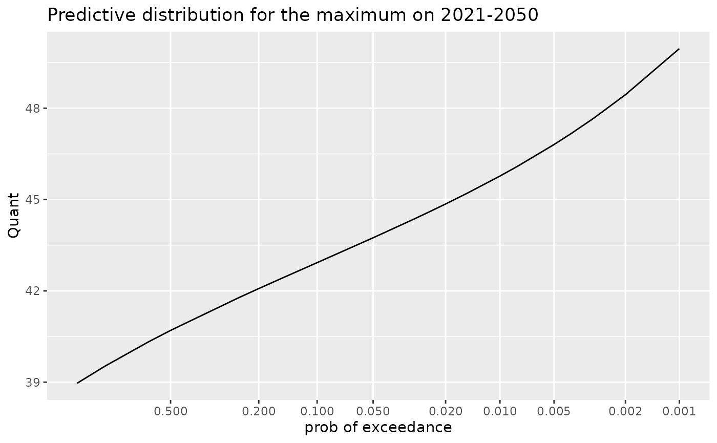
We can use the newTimeRange argument of the method predict for the class "TVGEVBayes". With partial matching, we can simply use new =

myPred <- predict(fit, new = "2021_2050")
tail(myPred)

##    newTimeRange  Prob    Quant
## 15    2021_2050 0.008 46.08961
## 16    2021_2050 0.005 46.80702
## 17    2021_2050 0.004 47.17385
## 18    2021_2050 0.003 47.67545
## 19    2021_2050 0.002 48.44431
## 20    2021_2050 0.001 49.95837

Again a plot is drawn by using autoplot.

autoplot(myPred) + ggtitle("Predictive distribution for the maximum on 2021-2050")

MCMC diagnostics

It is a good practice to carefully inspect the MCMC iterates provided by Stan. For that aim, the excellent Shiny interface provided by the shinystan package is of great help.

library(shinystan)
my_sso <- launch_shinystan(fit$stanFit)

This chunk (not executed here) lauches the Shiny interface in the web browser. This allows to get interactively: traceplots and scatterplots for the parameters, convergence disagnostics, and much more.

Censored data, historical data

Censoring by interval

Beside the Bayesian inference the TVGEVBayes function allows the use of observations that are censored, more precisely: censored by interval. Instead of the exact value $y_t$ for the time (year) $t$ , we only know that the observation for a given year falls in an interval $(y_{\text{L},t}, \, y_{\text{U},t})$ . Consequently the contribution of year $t$ in the likelihood $\log L_t = F_{\text{GEV}}(y_{\text{U},t};\, \boldsymbol{\psi}) - F_{\text{GEV}}(y_{\text{L},t};\, \boldsymbol{\psi}).$ We can take $y_{\text{L},t} = -\infty$ or $y_{\text{U},t} = \infty$ using the Inf special number in R.

This kind of information can be given in TVGEVBayes by using the optional timeMAXdata argument and giving as value an object with class "timeMAXdata" constructed with creator function of the same name. For instance it is believed that annual maximum for year 1922 in Dijon-Longvic was $\geq 34.4$ C since the last value was recorded on 1922-05-24.

tMD <- timeMAXdata("1922_1922" = list("1922-05-24" = c(34.4, Inf)))
class(tMD)

## [1] "timeMAXdata"

A natural way to represent such censored observations is to plot them as a vertical segment rather than a point.

autoplot(tMD) + theme_gray() + ggtitle("timeMAXdata censored data")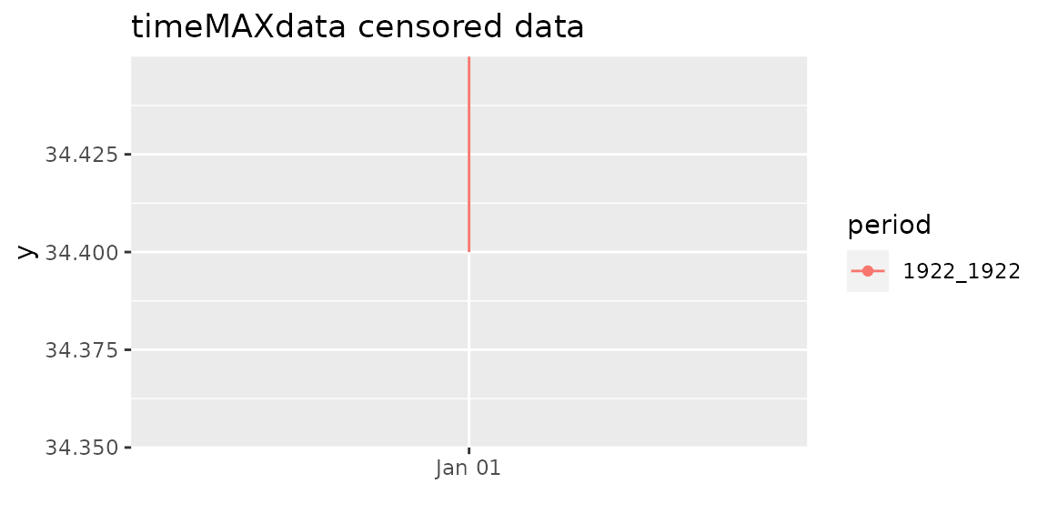

A segment reaching the limit of the plotting area should be considered as possibly having an infinite bound as here.

fitCens <- TVGEVBayes(data = df,
                      date = "Date", response = "TXMax",
                      timeMAXdata = tMD,
                      design = breaksX(date = Date, breaks = "1970-01-01", degree = 1),
                      loc = ~ t1 + t1_1970, scale = ~ 1, shape = ~ 1,
                      seed = 1234)
summary(fitCens)
autoplot(fitCens) + theme_gray() +
    ggtitle("Posterior mean for the GEV expectation")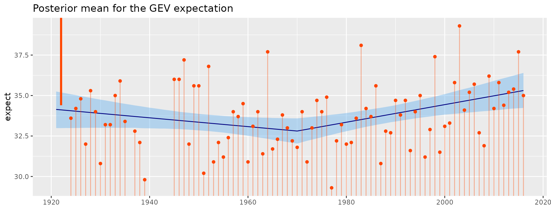

autoplot(fitCens, which = "quantile", prob = 0.95) + theme_gray() +
    ggtitle("Posterior mean for the  GEV quantile with probability 0.95")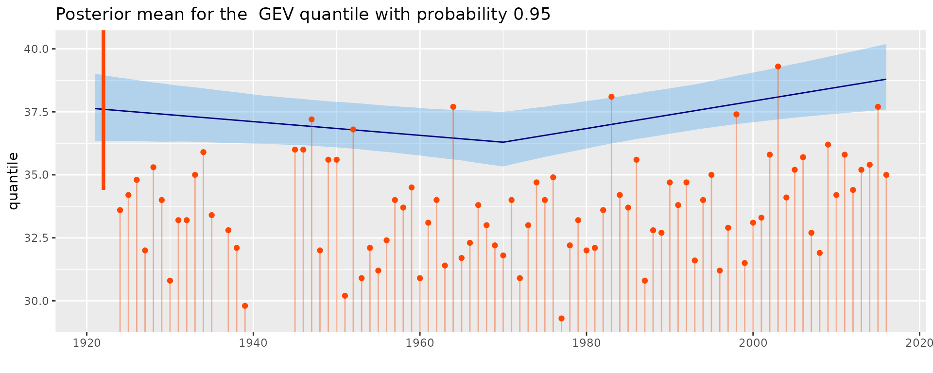

timeMaxdata objects

The name "timeMAXdata" is formed after MAXdata of the Renext package, although it is quite different. A timeMAXdata object specifies a number of periods or time ranges given in the creator through names as in a list call. The names used must define time ranges (or periods) with the syntax begin_end. The corresponding value is itsel a list, with named elements corresponding to the largest values on the time range. The name of an element is a character string defining a date, and its value is a vector of length 1 or 2. In the first case the known (uncensored) value is given and in the second case, the observation is censored and the two limits (possibly infinite) ar given.

tMD <- timeMAXdata("1922_1922" = list("1922-05-24" = c(34.4, Inf)))

Time ranges or periods, dates

The time ranges are given as begin_end, where begin and end are year or date.

tMD <- timeMAXdata("1922_1930" = list("1922-05-24" = c(34.4, Inf),
                       "1927-08-01" = c(36.0, 37.0)))
autoplot(tMD) + theme_gray() + ggtitle("Illustrative timeMAXdata")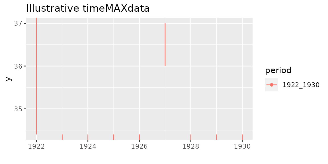

The provided information is for the years 1922 to 1930 ( $9$ years). We tell that the two largest observations are for years 1922 and 1927 and (optionally) provide the full date. In both case the observations are censored by interval. By affirming that these are the two largest observations, we tell that the $7$ remaining observations are certainly below, so are below $34.4$ . So these observations will be considered as censored with bounds $-\infty$ and $34.4$ .

A timeMAXdata object can similarly contain several periods which should not intersect. Note that a key function is the byBloc which aggregates the information by block, with a default block duration of one year.

byBlock(tMD)

##      period       date  y   yL   yU
## 1 1922_1930 1922-01-01 NA 34.4  Inf
## 2 1922_1930 1923-01-01 NA   NA 34.4
## 3 1922_1930 1924-01-01 NA   NA 34.4
## 4 1922_1930 1925-01-01 NA   NA 34.4
## 5 1922_1930 1926-01-01 NA   NA 34.4
## 6 1922_1930 1927-01-01 NA 36.0 37.0
## 7 1922_1930 1928-01-01 NA   NA 34.4
## 8 1922_1930 1929-01-01 NA   NA 34.4
## 9 1922_1930 1930-01-01 NA   NA 34.4

byBlock(tMD, blockDuration ="2 years")

##      period       date  y   yL   yU
## 1 1922_1930 1922-01-01 NA 34.4  Inf
## 2 1922_1930 1924-01-01 NA   NA 34.4
## 3 1922_1930 1926-01-01 NA 36.0 37.0
## 4 1922_1930 1928-01-01 NA   NA 34.4

Note that there are major differences with the MAXdata structure of Renext

A timeMAXdata does not embed a variable name. The related variable is automatically named y so that yLand yU are lower and upper bounds.
If several observations are given for a same year, an error is cast when using byBlock

tMD <- timeMAXdata("1922_1930" = list("1922-05-24" = c(34.4, Inf),
                       "1922-08-01" = c(36.0, 37.0)))
try(byBlock(tMD))

## Error in byBlock(tMD) : 
##   'Several MAXdata obs. in the same block. Not allowed yet.

Also note that there are some inconsistencies in the vocabulary because in Renext MAXdata a block is to be undestood as a time range for which the max observations are provided, whatever be the duration of this time range. Finally, MAXdata can not contain censored observations.

Yves Deville deville.yves@alpestat.com