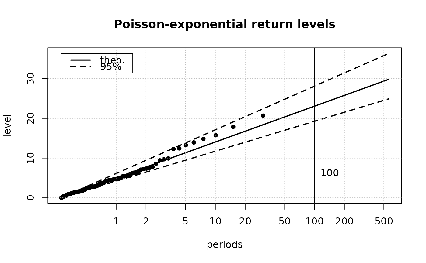
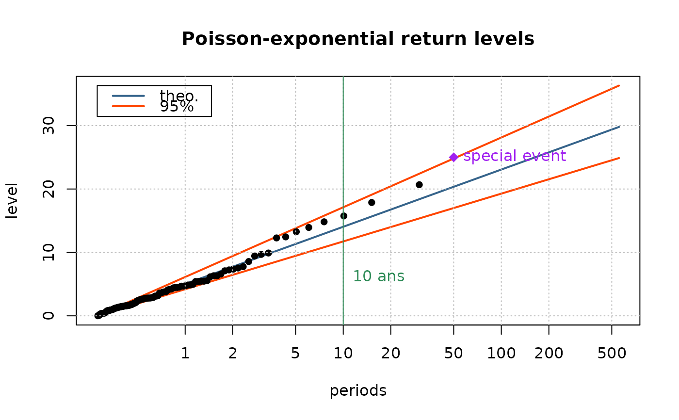
Return level plot

Return level plot for "Renouvellement" data.

Usage

RLplot(data,
       x = NULL,
       duration = 1,
       lambda,
       conf.pct = 95,
       mono = TRUE,
       mark.rl = 100,
       mark.labels = mark.rl,
       mark.col = NULL,
       main = NULL,
       ylim = NULL,
          ...)

Arguments

data

A data.frame object with a column named quant.

x

Optional vector of observed levels.

duration

The (effective) duration corresponding to x if this argument is used.

lambda

Rate, with unit inverse of that used for duration, e.g. in inverse years when duration is in years.

conf.pct

Vector (character or integer) giving confidence levels. See Details below.

mono

If TRUE colours are replaced by black.

mark.rl

Return levels to be marked on the plot.

mark.labels

Labels shown at positions in mark.rl.

mark.col

Colours for marked levels.

main

Main title for the return level plot (defaults to empty title).

ylim

Limits for the y axis (defaults to values computed from the data).

...

Further args to be passed to plot. Should be removed in future versions.

Details

Percents should match column names in the data.frame as follows. The upper and lower limits are expected to be U.95 and L.95 respectively. For a 70% confidence percentage, columns should have names "U.70" and "L.70".

The plot is comparable to the return level described in Coles'book and related packages, but the return level is here in log-scale while Coles uses a loglog-scale. A line corresponds here to a one parameter exponential distribution, while Coles'plot corresponds to Gumbel, however the two plots differ only for small return periods. This plot is identical to an expplot but with x and y scales changed: only axis tick-marks differ. The convexity of the scatter plot is therefore opposed in the two plots.

References

Coles S. (2001) Introduction to Statistical Modelling of Extremes Values, Springer.

Author

Yves Deville

Note

Confidence limits correspond to two-sided symmetrical intervals. This means that the (random) confidence interval may be under or above the true unknown value with the same probabilities. E.g. the probability that the unknown quantile falls above U.95 is 2.5%. The two bounds are yet generally not symmetrical with respect to quant; such a behaviour follows from the use of "delta" method for approximate intervals.

It is possible to add graphical material (points, lines) to this plot using log(returnlev) and quantile coordinates. See Examples section.

Examples

## Typical probability vector
prob <- c(0.0001,
  seq(from = 0.01, to = 0.09, by = 0.01),
  seq(from = 0.10, to = 0.80, by = 0.10),
  seq(from = 0.85, to = 0.99, by = 0.01),
  0.995, 0.996, 0.997, 0.998, 0.999, 0.9995)

## Model parameters rate = #evts by year, over nyear
lambda <- 4
nyear <- 30
theta.x <- 4

## draw points
n.x <- rpois(1, lambda = lambda*nyear)
x <- rexp(n.x, rate = 1/theta.x)

## ML estimation (exponential)
lambda.hat <- n.x / nyear
theta.x.hat <- mean(x)
  
## Compute bounds (here exact)
alpha <- 0.05

quant <- qexp(p = prob, rate = 1/theta.x.hat) 

theta.L <- 2*n.x*theta.x.hat / qchisq(1 - alpha/2, df = 2*n.x)
theta.U <- 2*n.x*theta.x.hat / qchisq(alpha/2, df = 2*n.x)

L.95 <- qexp(p = prob, rate = 1/theta.L) 
U.95 <- qexp(p = prob, rate = 1/theta.U) 

## store in data.frame object
data <- data.frame(prob = prob, quant = quant, L.95 = L.95, U.95 = U.95)

RLplot(data = data, x = x, lambda = lambda.hat,
       duration = nyear,
       main = "Poisson-exponential return levels")


RLplot(data = data, x = x, lambda = lambda.hat, duration = nyear,
       mark.rl = 10, mark.labels = "10 ans", mono = FALSE, mark.col = "SeaGreen",
       main = "Poisson-exponential return levels")

points(x = log(50), y = 25, pch = 18, cex = 1.4, col = "purple") 
text(x = log(50), y = 25, col ="purple", pos = 4, labels = "special event")