Poisson-GP Model with Bayesian Inference Results

Create an object representing a Poisson-GP model with Bayesian inference result using the revdbayes package.

Usage

poisGPBayes(data, threshold, effDuration,
            a0 = 1, b0 = 0,
            priorGP = "flatflat",
            lowerGP = c("scale" = 0, "shape" = -0.9),
            upperGP = c("scale" = Inf, "shape" = Inf),
            trace = 0)

Arguments

data: Numeric vector containing the marks.
threshold: The threshold.
effDuration: The effective duration of the observation period.
a0, b0: Shape and rate for a gamma prior on the Poisson rate lambda. Note that by choosing a0 = 1 and b0 = 0 we define an improper flat prior on \((0, \infty)\). While a0 is dimensionless and compares to \(1 +\) a number of observations, b0 has the dimension of a duration and compares to a duration of observation.
priorGP: A character defining which prior is used for the GP part of the model as in the revdbayes package.
lowerGP, upperGP: Bounds on the GP parameters.
trace: Level of verbosity.

Value

An object with S3 class "poisGPBayes".

Details

@details This function mainly relies on the revdbayes package which is used to produce the results of the Bayesian inference using MCMC. However the Maximum A Posteriori (MAP) for the parameter vector is computed by maximising the posterior function using a numerical optimisation. This allows a better comparison with the frequentist ML approach as used in poisGP.

Examples

## ========================================================================
## Use the Garonne data from Renext
## ========================================================================
fit <- poisGPBayes(data = Garonne$OTdata$Flow,
                   threshold = 2500, effDuration = 64)
#> Warning: 'threshold' is smaller than the smallest observation

## ========================================================================
## Some S3 methods: RL for Return Levels, ...
## ========================================================================
class(fit)
#> [1] "poisGPBayes"
coef(fit)
#>        lambda    scale      shape
#> mode 2.359557 1239.904 -0.1356296
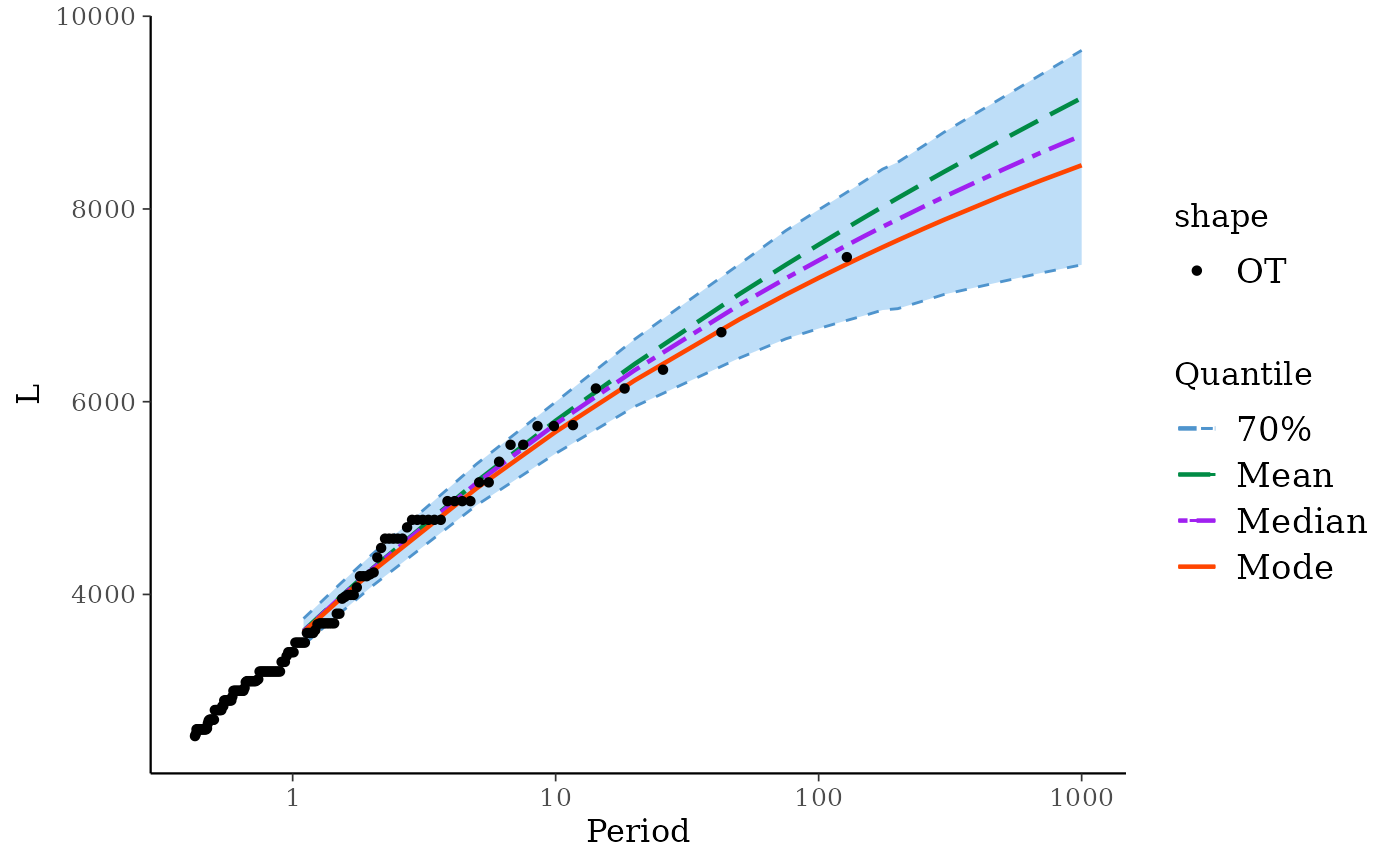
RL(fit)
#>    Period Level     Mode   Median     Mean        L        U
#> 1     1.1   70% 3609.303 3618.069 3622.249 3475.020 3749.386
#> 2     1.5   70% 3940.193 3954.955 3960.563 3795.332 4098.430
#> 3     2.0   70% 4234.910 4259.698 4264.141 4083.407 4413.235
#> 4     5.0   70% 5100.513 5154.605 5170.913 4925.161 5352.844
#> 5    10.0   70% 5687.450 5768.397 5802.284 5462.380 5997.135
#> 6    20.0   70% 6221.722 6327.763 6392.509 5950.471 6649.227
#> 7    50.0   70% 6855.138 7004.816 7117.486 6453.699 7427.608
#> 8    75.0   70% 7111.266 7279.590 7420.467 6652.257 7775.053
#> 9   100.0   70% 7284.637 7466.466 7629.417 6758.908 7991.787
#> 10  125.0   70% 7414.531 7608.647 7788.237 6835.766 8155.347
#> 11  150.0   70% 7517.783 7722.144 7915.980 6895.842 8292.896
#> 12  175.0   70% 7603.111 7815.592 8022.615 6951.127 8413.295
#> 13  200.0   70% 7675.597 7892.799 8114.001 6965.566 8485.049
#> 14  250.0   70% 7793.836 8023.002 8264.737 7046.091 8654.157
#> 15  300.0   70% 7887.824 8125.949 8386.124 7113.225 8797.124
#> 16  500.0   70% 8139.108 8406.377 8718.208 7248.326 9156.076
#> 17  700.0   70% 8295.364 8584.671 8930.920 7335.337 9394.395
#> 18 1000.0   70% 8453.398 8762.482 9151.588 7420.329 9645.842
autoplot(fit)
#> Warning: Since 'data' has class "potData" the formal arguments 'effDuration', 'nOT', 'MAX.*' and 'OTS.*' are ignored
#> Warning: 'threshold' is smaller than the smallest observation
#> Scale for x is already present.
#> Adding another scale for x, which will replace the existing scale.