Density, Distribution Function, Quantile Function and Random Generation for the Five-Parameter Compound Generalized Pareto Distribution (CGPD)
CGPD.RdDensity, distribution function, quantile function and random generation for the five-parameter Compound Generalized Pareto Distibution (CGPD).
Usage
dCGPD(x, loc = 0.0, scale = 1.0, shape = 0.0,
      scaleN, shapeN, EN, IDN, log = FALSE)

pCGPD(q, loc = 0.0, scale = 1.0, shape = 0.0,
      scaleN, shapeN, EN, IDN, lower.tail = TRUE)

qCGPD(p, loc = 0.0, scale = 1.0, shape = 0.0,
      scaleN, shapeN, EN, IDN, lower.tail = TRUE)

rCGPD(n, loc = 0.0, scale = 1.0, shape = 0.0,
      scaleN, shapeN, EN, IDN)

pCGPD(
  q,
  loc = 0,
  scale = 1,
  shape = 0,
  scaleN,
  shapeN,
  EN,
  IDN,
  lower.tail = TRUE
)

qCGPD(
  p,
  loc = 0,
  scale = 1,
  shape = 0,
  scaleN,
  shapeN,
  EN,
  IDN,
  lower.tail = TRUE
)

rCGPD(n, loc = 0, scale = 1, shape = 0, scaleN, shapeN, EN, IDN)
Arguments
- x, q
Vector of quantiles.
- loc
Location parameter. Numeric vector of length one.
- scale
Scale parameter. Numeric vector of length one.
- shape
Shape parameter. Numeric vector of length one.
- scaleN
Scale of the GPD for the \(N\) part. Along with
shapeNit provides the parameterisation for the Binomial-Poisson-Negative Binomial familly.- shapeN
Shape of the GPD for the \(N\) part. Along with
scaleNit provides the parameterisation for the Binomial-Poisson-Negative Binomial familly.- EN
Expectation of \(N\). Along with
IDNit provides an alternative parameterisation for the \(N\) part.- IDN
Index of Dispersion of \(N\). Along with
ENit provides an alternative parameterisation for the \(N\) part.- log
Logical; if
TRUE, densitiespare returned aslog(p).- lower.tail
Logical; if
TRUE(default), probabilities are P[X <= x], otherwise, P[X > x].- p
Vector of probabilities.
- n
Sample size.
Details
This distribution is that of the maximum \(M\) of \(N\) i.i.d. r.vs \(X_i\) with distribution \(\textrm{GPD}(\mu,\,\sigma,\,\xi)\) where \(N\) is a r.v. with non-negative integer values, independent of the sequence \(X_i\), and having a Binomial, Poisson or Negative Binomial distribution. The distribution of \(N\) can be parameterized by using two parameters \(\mu_N\) and \(\sigma_N\) in a GPD style, or alternatively by using the two parameters \(\mathrm{E}(N)\) and \(\textrm{ID}(N)\) representing the expectation and the index of dispersion of \(N\). The three cases Binomial, Poisson and Negative Binomial correspond to \(\textrm{ID}_N < 0\), \(\textrm{ID}_N = 0\) and \(\textrm{ID}_N > 0\).
Caution
This distribution is of mixed-type. It
has a probability mass at \(-\infty\) corresponding to the
possibility that \(N=0\) in which case \(M\) is the maximum of
an empty set, taken as \(-\infty\) corresponding to
max(mumeric(0)). Consequently a sample drawn by using
rCGPD contains -Inf values with positive
probability.
References
Yves Deville (2019) "Bayesian Return Levels in Extreme-Value Analysis" IRSN technical report.
Examples
set.seed(1)
ExpN <- runif(1)
IDN <- rexp(1, rate = 1)
scaleN <- 1 / ExpN
shapeN <- (IDN - 1) / ExpN
loc <- rnorm(1, mean = 0, sd = 10); scale <- rexp(1)
shape <- rnorm(1 , mean = 0, sd = 0.1)
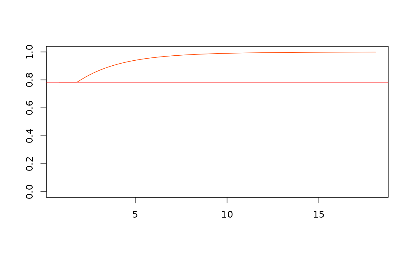
mass <- pCGPD(-Inf, scaleN = scaleN, shapeN = shapeN,
loc = loc, scale = scale, shape = shape)
q <- qCGPD(p = c(mass + 0.001, 0.999), scaleN = scaleN, shapeN = shapeN,
loc = loc, scale = scale, shape = shape)
x <- seq(from = q[1] - 1, to = q[2], length.out = 200)
F <- pCGPD(x, scaleN = scaleN, shapeN = shapeN,
loc = loc, scale = scale, shape = shape)
plot(x, F, type = "l", xlab = "", ylab = "", ylim = c(0, 1),
col = "orangered")
abline(h = mass, col = "red")
 f <- dCGPD(x, scaleN = scaleN, shapeN = shapeN,
loc = loc, scale = scale, shape = shape)
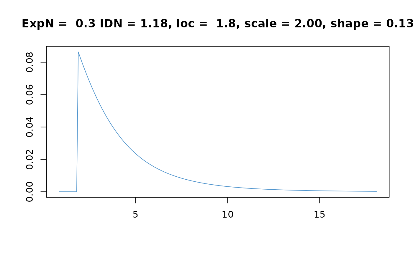
plot(x, f, type = "l", col = "SteelBlue3", xlab = "", ylab = "")
title(main = sprintf(paste("ExpN = %4.1f IDN = %4.2f,",
"loc = %4.1f, scale = %4.2f, shape = %4.2f"),
ExpN, IDN, loc, scale, shape))
f <- dCGPD(x, scaleN = scaleN, shapeN = shapeN,
loc = loc, scale = scale, shape = shape)
plot(x, f, type = "l", col = "SteelBlue3", xlab = "", ylab = "")
title(main = sprintf(paste("ExpN = %4.1f IDN = %4.2f,",
"loc = %4.1f, scale = %4.2f, shape = %4.2f"),
ExpN, IDN, loc, scale, shape))