Simulate a random RenData object

Simulate a random RenData object that can be used within the Renouv function for tests.

Usage

rRendata(lambda = 1,
         threshold = 0,
         effDuration = 100,
         distname.y = "exp",
         par.y = c(rate = 1),
         start = "1913-01-01",
         name = NULL,
         varName = "X", varUnit = "?",
         simDate = TRUE, roundDate = FALSE,
         MAX.effDuration = NULL,
         MAX.r = rep(1L, length(MAX.effDuration)),
         OTS.effDuration = NULL,
         OTS.threshold = NULL)

Arguments

lambda

The rate of the Homogeneous Poisson Process.

threshold

The threshold for the exceedances.

effDuration

The effective duration of the main Over Threshold (OT) period. This must be a positive value.

distname.y

Name of the distribution for the excesses to be simulated. See Details.

par.y

A named vector or list giving the parameters values for the distribution. The name must conform to the chosen distribution.

start

A POSIXct object, or character that can be coerced to POSIXct (e.g. a date given as a character in the "YYYY-MM-DD" format) giving the start of the main OT sample.

name

A name for the dataset which will be attached to it and be used by some methods for "Rendata".

varName

Name of the simulated variable.

varUnit

Unit for the simulated variable (is used by plot).

simDate

Logical. If TRUE the dates will be reported for the historical data (MAX and OTS).

roundDate

Logical. If TRUE the time part ot the date column will be rounded. Not implemented yet.

MAX.effDuration

Vector of the durations for the MAX historical blocks.

MAX.r

Vector of the (positive) numbers of observations for MAX historical blocks. Must have the same length as MAX.effDuration. See Caution below for the effect of selection large values.

OTS.effDuration

Vector of durations for the OTS historical blocks.

OTS.threshold

Vector of numerical thresholds for the observations in OTS historical blocks. Must have the same length as OTS.effDuration. All values must be >= threshold.

Details

The distribution of the excesses named in distname.y can be any known distribution, provided that when prefixed with the usual "r" letter, the name gives the wanted simulation function. For example, with distname.y = "exp", the rexp function is used and par.y must thus contain an element with name "rate".

When a suitable numeric threshold is given, the simulated marks of the marked process are the sum of the threshold and of a random excess drawn from distname.y. When the threshold is not a finite numeric value, the observed marks are the simulated values themselves.

The main OT sample is assumed to begin at start. Historical MAX blocks (if any) are assumed to be just before start, and OTS are just before start or just before the beginning of the MAX blocks when there are some. The dates are computed without taking into consideration the problems of leap years or leap seconds.

Value

An object with S3 class "Rendata". This class currently has

plot and summary methods.

Author

Yves Deville

Note

When effDuration is small relative to the inverse of lambda the number of simulated marks in the OT sample may be \(0\) which can cause problems for some uses of the created data.

Caution

By construction, each MAX block contains at least one observation, while a random period of the same duration might have none. The simulated number of events on a MAX block is generated using a censored Poisson distribution. Care must be taken when estimations are made on such data, since creating MAX blocks obviously create a positive bias on lambda. Such bias then also affects the other parameters concerning the excesses, because these parameters are no longer orthogonal to the rate parameter lambda when historical data are used. The bias can be severe if MAX blocks with small durations are used, or if large number of events are chosen in MAX.r.

Examples

set.seed(1234)
rd <- rRendata(effDuration = 60,
               MAX.effDuration = rep(3, 6),
               MAX.r = rep(4, 6),
               distname.y = "exp", par.y = c(rate = 1/100))
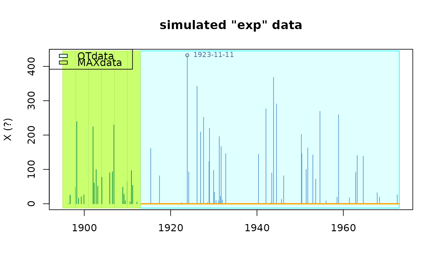
plot(rd)

summary(rd)
#> o Dataset simulated "exp" data
#>    data 'simulated "exp" data', variable 'X' (?) 
#> 
#> o OT data (main sample) from  1913-01-01  to  1972-12-17  (eff. dur.  60.00 years)
#>  
#>           n        Min.     1st Qu.      Median        Mean     3rd Qu. 
#>  50.0000000   0.6510342  14.1203716  91.9701602 114.8248081 165.6590278 
#>        Max. 
#> 432.4563092 
#> 
#> o no missing OT periods 
#> 
#> o 'MAX' historical info: 6 blocks, 24 obs., total duration = 18.00 years 
#> 
#> o no 'OTS' historical data 
#> 
rd2 <- rRendata(effDuration = 10,
                MAX.effDuration = rep(60, 2),
                MAX.r = rep(3, 2),
                simDate = FALSE,
                distname.y = "gpd", par.y = c(scale = 20, shape = 0.16))
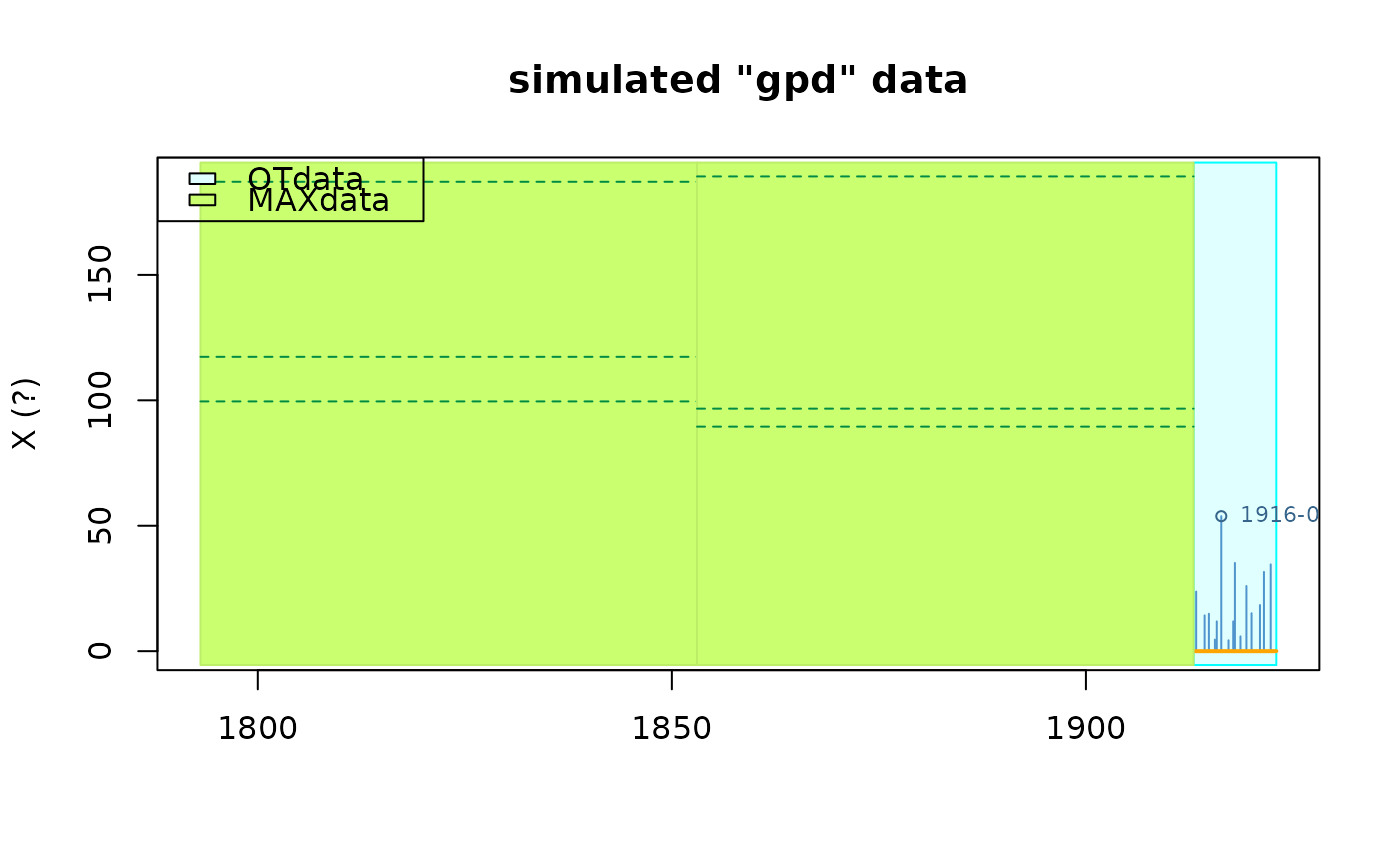
plot(rd2)

rd3 <- rRendata(effDuration = 10,
                OTS.effDuration = rep(60, 2),
                OTS.threshold = rep(80, 2),
                simDate = FALSE,
                distname.y = "gpd", par.y = c(scale = 20, shape = 0.16))
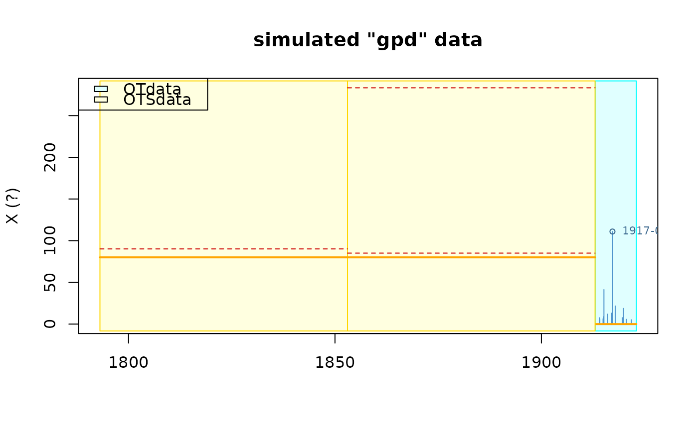
plot(rd3)

## Renouv fit with historical data
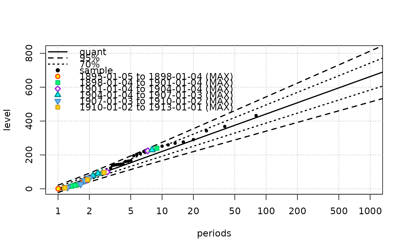
fit <- Renouv(rd)

summary(fit)
#> o Main sample 'Over Threshold'
#>     . Threshold            0.00
#>     . Effect. duration    60.00 years
#>     . Nb. of exceed.      50
#> 
#> o Estimated rate 'lambda' for Poisson process (events):  1.00 evt/year.
#> 
#> o Distribution for exceedances y: "exponential", with 1 par. "rate" 
#> 
#> o No transformation applied
#> 
#> o Coefficients
#> 
#>          Estimate  Std. Error  t value
#> lambda 0.99752850 0.116045914 8.595981
#> rate   0.01042349 0.001200677 8.681345
#> 
#> Degrees of freedom: 2 (param.) and 74 (obs)
#> 
#> o Inference method used for return levels
#> "Delta method"
#> 
#> o Return levels
#> 
#>    period quant L.95 U.95 L.70 U.70
#> 24     10   221  167  274  192  249
#> 30     20   287  220  355  251  323
#> 34     50   375  288  462  329  421
#> 36    100   442  340  543  388  495
#> 38    200   508  392  624  447  569
#> 41    300   547  422  672  481  613
#> 43    400   575  444  705  505  644
#> 44    500   596  461  731  524  668
#> 46    600   613  474  753  540  687
#> 47    700   628  486  771  553  704
#> 48    800   641  496  787  564  718
#> 49    900   652  504  800  574  731
#> 50   1000   662  512  813  583  742
#> 
#> 
#> o 'MAX' historical info: 6  blocks, 24 obs., total duration = 18.00 years
#> 
#> o no 'OTS' historical data
#> 
#> o Kolmogorov-Smirnov test
#> 
#> 	Exact one-sample Kolmogorov-Smirnov test
#> 
#> data:  OTjitter(y.OT, threshold = 0)
#> D = 0.18402, p-value = 0.05916
#> alternative hypothesis: two-sided
#> 
#> 
#> o Implied model for block maxima
#>   Distribution: gumbel 
#>   Coeffficients
#>        loc      scale 
#> -0.2374022 95.9371765