ML estimation of a 'maxlo' distribution

Fast Maximum Likelihood estimation of a 'maxlo' distribution.

Usage

fmaxlo(x,
       shapeMin = 1.25,
       info.observed = TRUE,
       plot = FALSE,
       scaleData = TRUE,
       cov = TRUE)

Arguments

x

Sample vector to be fitted. Should contain only positive non-NA values.

shapeMin

Lower bound on the shape parameter. This must be >= 1.0 since otherwise the ML estimate is obtained with the scale parameter equal to max(x).

info.observed

Should the observed information matrix be used or the expected one be used?

plot

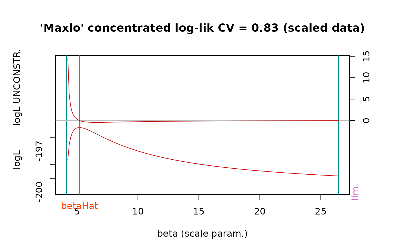
Logical. If TRUE, a plot will be produced showing the derivative of the concentrated log-likelihood, function of the shape parameter. The derivative function shown is that of the log-likelihood for the unconstrained maximisation; it is not used in the estimation.

scaleData

Logical. If TRUE observations in x (which are positive) are divided by their mean value. The results are in theory not affected by this transformation, but scaling the data could improve the estimation in some cases. The log-likelihood plots are shown using the scaled values so the returned estimate of the scale parameter is not the the abscissa of the maximum shown on the plot.

cov

Logical. If FALSE, a minimal estimation is performed with no covariance matrix or derivative returned. This can be useful when a large number of ML estimations are required, e.g. to sample from a likelihood ratio.

Details

The 'maxlo' likelihood is concentrated with respect to the shape parameter, thus the function to be maximised has only one one scalar argument: the scale parameter \(\beta\). For large scale \(\beta\), the derivative of the concentrated log-likelihood tends to zero, and its sign is that of \((\textrm{CV}^2-1)\) where \(\textrm{CV}\) is the coefficient of variation, computed using \(n\) as denominator in the formula for the standard deviation.

The ML estimate does not exist when the sample has a coefficient of variation CV greater than 1.0 and it may fail to be found when CV is smaller than yet close to 1.0.

The expected information matrix can be obtained by noticing that when the r.v. \(Y\) follows the 'maxlo' distribution with shape \(\alpha\) and scale \(\beta\) the r.v \(V:= 1/(1-Y/\beta)\) follows a Pareto distribution with minimum 1 and and shape parameter \(\alpha\). The information matrix involves the second order moment of \(V\).

The default value of info.observed was set to TRUE from version 3.0-1 because standard deviations obtained with this choice are usually better.

Value

A list with the following elements

estimate

Parameter ML estimates.

sd

Vector of (asymptotic) standard deviations for the estimates.

loglik

The maximised log-likelihood.

dloglik

Gradient of the log-likelihood at the optimum. Its two elements should normally be close to zero.

cov

The (asymptotic) covariance matrix computed from theoretical or observed information matrix.

info

The information matrix.

Author

Yves Deville

Note

The name of the distribution hence also that of the fitting function are still experimental and might be changed.

Examples

## generate sample
set.seed(1234)
n <- 200
alpha <- 2 + rexp(1)
beta <- 1 + rexp(1)
x <- rmaxlo(n, scale = beta, shape = alpha)
res <- fmaxlo(x, plot = TRUE)


## compare with a GPD with shape 'xi' and scale 'sigma'
xi <- -1 / alpha; sigma <- -beta * xi
res.evd <- evd::fpot(x, threshold = 0, model = "gpd")
xi.evd <- res.evd$estimate["shape"]
sigma.evd <- res.evd$estimate["scale"]
beta.evd <- -sigma.evd / xi.evd 
alpha.evd <- -1 / xi.evd
cbind(Renext = res$estimate, evd = c(alpha = alpha.evd, beta = beta.evd))
#>         Renext      evd
#> shape 4.204632 4.204418
#> scale 1.175853 1.175803