Barplot for Renouv "Over Threshold" counts

Barplot for "Over Threshold" counts in time blocks (usually years)

Usage

barplotRenouv(data,
               blockname = colnames(data)[1],
               varname = colnames(data)[2],
               threshold = quantile(data[, varname], 0.2),
               na.block = NULL,
               plot = TRUE,
               main = NULL, xlab = NULL, ylab = NULL,
               mono = FALSE,
               prob.theo = 0.999,
               ...)

Arguments

data

A dataframe object containing the variables.

blockname

Name of the "block" variable (column in data). This variable should contain integers, or be of class "factor", but with integer values such as year numbers.

varname

Name of the variable (e.g. "Surge").

threshold

Only obs for which the variable exceeds threshold will be taken into account.

na.block

Values of blocks containing missing values. See the Details section.

plot

If FALSE tests are computed without producing any plot.

main

Character for main title or NULL in which case a default main title is used.

xlab

Character for x axis label or NULL in which case a default lab is used.

ylab

Character for y axis or NULL in which case a default lab is used.

mono

If FALSE barplot will have colors, else greyscale will be used.

prob.theo

The total theoretical probability corresponding to the plotted (theoretical) bars.

...

Further args to be passed to barplot.

Details

Blocks described in the na.block are omitted in the determination of counts. The object given in the na.block is coerced to character and the same is done for values of block before comparing them to the na.block values. If block variable is of class factor with levels representing years (e.g. 1980, 1981, etc.) missing blocks can be specified either as c("1980", "1981") or as numeric c(1980, 1981).

For the chi-square test, counts for neighbouring frequency classes are grouped in order to reach a minimum frequency of 5 in each group. E.g. if we expect respectively 1.0, 3.8 and 7.0 blocks with frequency 0, 1 and 2 for events, the three counts are grouped in one group with frequency 1.0+3.8+7.0=11.8. Note that this strategy of grouping is not unique and is likely to weaken the power of the test. Before grouping, the higher class theoretical probability is computed as the probability to obtain a count equal to or greater than the max value.

Value

A list with the following objects.

freq

frequency table (matrix) giving observed and theoretical (Poisson) frequencies as well as a group number for the chi-square test.

overdispersion

the overdispersion coefficient (variance/mean ratio).

disp.test

a list giving results of the (over)dispersion test. See the reference Yagouti and al. in the References section.

chisq.test

a list giving results for the chis-square test of goodness-of-fit to the Poisson distribution.

tests

a matrix with the two tests displayed in two rows.

For both tests, the statistic follows a chi-square distribution under the null hypothesis . The list of results contains the statistic

statistic, the number of degrees of freedom df and the \(p\)-value p.value.

References

See Yagouti A., Abi-Zeid I., Ouarda, T.B.M.J. and B. Bobée (2001), Revue de processus ponctuels et synthèse de tests statistiques pour le choix d'un type de processus Revue des Sciences de l'Eau, 1, pp. 323-361.

Author

Yves Deville

Note

The two tests: (over-)dispersion and chi-square have one-sided (upper tail) \(p\)-value. In other words, we do not intend to reject when statistics take "abnormally small" values, but only when abnormally large values are met.

Examples

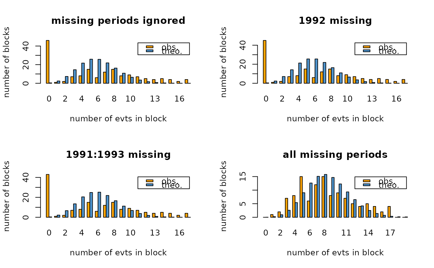
## na.block influence for Brest data
opar <- par(mfrow = c(2, 2))

bp1 <- barplotRenouv(data = Brest.years, threshold = 30,
         main = "missing periods ignored")
#> 
#> Goodness-of-fit test (Poisson). Stat = 277.1667 df = 8 p-value = 0 
#> 
#> Dispersion index 4.208457 p-value 0 
bp2 <- barplotRenouv(data = Brest.years, threshold = 30,
         na.block = 1992, main = "1992 missing")
#> number of obs. in NA blocks: 1 
#> 
#> Goodness-of-fit test (Poisson). Stat = 271.7896 df = 8 p-value = 0 
#> 
#> Dispersion index 4.170886 p-value 0 
bp3 <- barplotRenouv(data = Brest.years, threshold = 30,
         na.block = 1991:1993, main ="1991:1993 missing")
#> number of obs. in NA blocks: 3 
#> 
#> Goodness-of-fit test (Poisson). Stat = 261.2294 df = 8 p-value = 0 
#> 
#> Dispersion index 4.094299 p-value 0 
bp4 <- barplotRenouv(data = Brest.years, threshold = 30,
         na.block = Brest.years.missing, main = "all missing periods")
#> number of obs. in NA blocks: 46 
#> 
#> Goodness-of-fit test (Poisson). Stat = 30.97919 df = 8 p-value = 0.0001417065 
#> 
#> Dispersion index 1.791952 p-value 4.850723e-07 


par(opar)

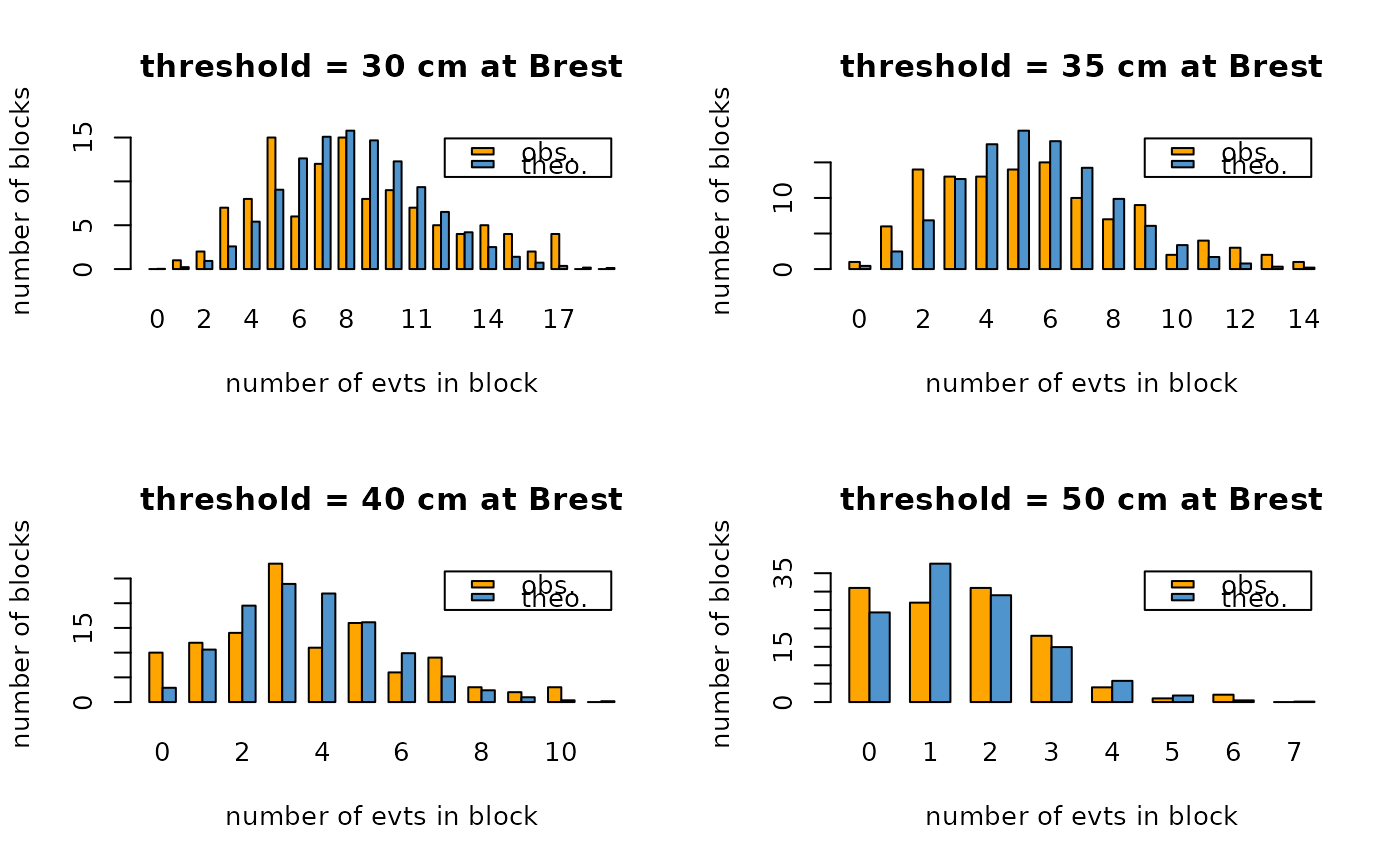
## threshold influence
opar <- par(mfrow = c(2,2))

thresh <- c(30, 35, 40, 50)

for (i in 1:length(thresh)) {
  bp  <- barplotRenouv(data = Brest.years, threshold = thresh[i],
                   na.block = Brest.years.missing,
                   main = paste("threshold =", thresh[i], "cm at Brest"))
}
#> number of obs. in NA blocks: 46 
#> 
#> Goodness-of-fit test (Poisson). Stat = 30.97919 df = 8 p-value = 0.0001417065 
#> 
#> Dispersion index 1.791952 p-value 4.850723e-07 
#> number of obs. in NA blocks: 46 
#> 
#> Goodness-of-fit test (Poisson). Stat = 24.5375 df = 7 p-value = 0.0009161369 
#> 
#> Dispersion index 1.740394 p-value 1.827177e-06 
#> number of obs. in NA blocks: 46 
#> 
#> Goodness-of-fit test (Poisson). Stat = 21.5105 df = 5 p-value = 0.000648504 
#> 
#> Dispersion index 1.605952 p-value 4.652672e-05 
#> number of obs. in NA blocks: 46 
#> 
#> Goodness-of-fit test (Poisson). Stat = 5.722912 df = 3 p-value = 0.1258975 
#> 
#> Dispersion index 1.159493 p-value 0.1181542 

par(opar)