Shifted Left Truncated Weibull (SLTW) distribution

Density function, distribution function, quantile function and random generation for the Shifted Left Truncated Weibull distribution.

Usage

dSLTW(x, delta = 1.0, shape = 1.0, scale = 1.0, log = FALSE)
   pSLTW(q, delta = 1.0, shape = 1.0, scale = 1.0, lower.tail = FALSE)
   qSLTW(p, delta = 1.0, shape = 1.0, scale = 1.0)
   rSLTW(n, delta = 1.0, shape = 1.0, scale = 1.0)

Arguments

x, q

Vector of quantiles.

p

Vector of probabilities.

n

Number of observations.

delta, shape, scale

Shift, shape and scale parameters. Vectors of length > 1 are not accepted.

log

Logical; if TRUE, the log density is returned.

lower.tail

Logical; if TRUE (default), probabilities are \(\textrm{Pr}[X \le x]\), otherwise, \(\textrm{Pr}[X > x]\).

Details

The SLTW distribution function with shape \(\alpha > 0\), scale \(\beta > 0\) and shift \(\delta > 0\) has survival function $$S(y) = \exp\left\{ -\left[ \left( \frac{y + \delta}{\beta} \right)^\alpha - \left( \frac{\delta}{\beta} \right)^\alpha \right] \right\} \qquad (y > 0) $$ This distribution is that of \(Y := X - \delta\) conditional to \(X > \delta\) where \(X\) follows a Weibull distribution with shape \(\alpha\) and scale \(\beta\).

The hazard and mean residual life (MRL) are monotonous functions with the same monotonicity as their Weibull equivalent (with the same shape and scale). The moments or even expectation do not have simple expression.

This distribution is sometimes called power exponential. It is occasionally used in POT with the shift delta taken as the threshold as it should be when the distribution for the level \(X\) (and not for the exceedance \(Y\)) is known to be the standard Weibull distribution.

Value

dSLTW gives the density function, pSLTW gives the distribution function, qSLTW

gives the quantile function, and rSLTW generates random deviates.

See also

Lomax for the Lomax distribution which is a limit case of SLTW.

Examples

shape <- rexp(1)+1  
delta = 10

xl <- qSLTW(c(0.001, 0.99), delta = delta, shape = shape)
x <- seq(from = xl[1], to = xl[2], length.out = 200)
f <- dSLTW(x, delta = delta, shape = shape)
plot(x, f, type = "l", main = "SLTW density")


F <- pSLTW(x, delta = delta, shape = shape)
plot(x, F, type = "l", main = "SLTW distribution")


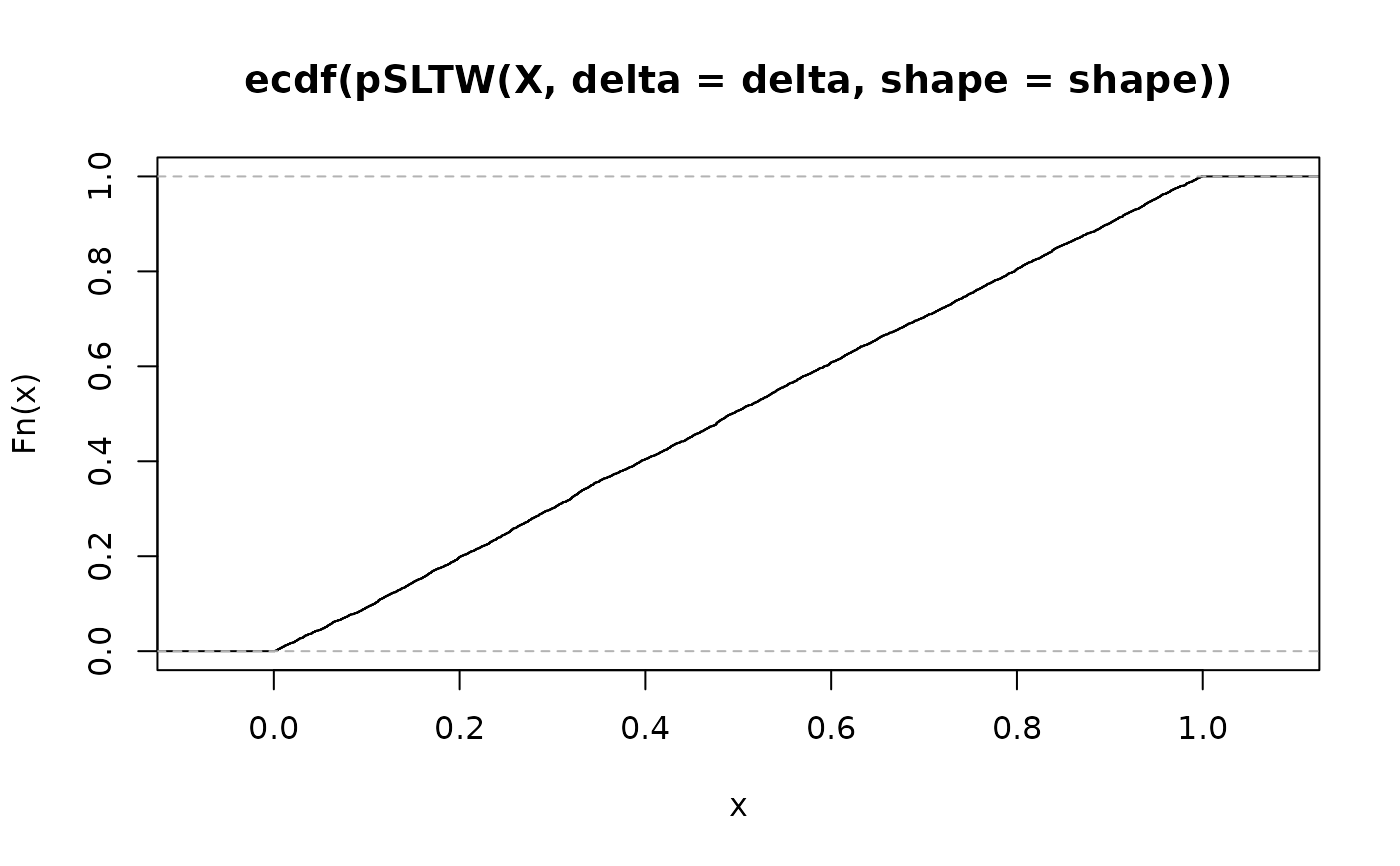
X <- rSLTW(5000, delta = delta, shape = shape)
## Should be close to the uniform repartition
plot(ecdf(pSLTW(X, delta = delta, shape = shape)))