Define a 'renouvellement' model without estimation

Build a 'renouvellement' model using parameters given by the user.

Usage

RenouvNoEst(threshold,
            estimate = NULL,
            distname.y = "exponential",
            fixed.par.y = NULL,
            trans.y = NULL,
            pct.conf = c(95, 70),
            rl.prob = NULL,
            prob.max = 1 - 1e-04,
            pred.period = NULL,
            cov = NULL,
            nb.OT = NULL,
            infer.method = NULL)

Arguments

threshold

The threshold.

estimate

Numeric named vector containing the estimates for the parameters. It must be compatible with the distribution chosen, and must contain in first position an element named "lambda" representing an estimated event rate in events by year.

distname.y

Character giving the name of the distribution.

fixed.par.y

Numeric named vector containing values for vectors which are considered as fixed (and not estimated).

trans.y

Transformation as in Renouv. Used only when distname.y is equal to "exponential".

pct.conf

Vector of percents for confidence limits.

rl.prob

Probability used in the return level computations. These values are used for instance in return level plots produced with the plot.Renouv method. When NULL a default vector is used.

prob.max

Maximal probability for which computations are done.

pred.period

Vector of periods for which predicted return levels will be computed.

cov

Covariance matrix for the provided estimated parameters. Must have rownames and colnames in accordance with those of estimate. This covariance matrix is used to build confidence limits on parameters and on return levels using the delta method.

nb.OT

Number of data over the threshold used for estimation. This will be used only when distname.y is equal to "exponential".

infer.method

Inference method. Will normally be the delta method.

Details

This function is used for plotting or comparing models with known parameter estimates but with no data available.

The parameters estimates should be accompanied with a covariance matrix assuming an approximately normal joint distribution of these. This matrix is usually obtained by computing the numerical derivatives of the log-likelihood at the second order at the estimates. This covariance is used to compute approximate confidence limits for the return levels of the unknown true distribution that was estimated.

Value

An object of class "Renouv" representing a 'renouvellement' model similar to those built with Renouv. This is mainly a list. Note however that some list elements found in Renouv

objects built by Renouv can not be found here. For instance, the returned objects embeds no goodness-of-fit results since the object is created without making use of any data.

Author

Yves Deville

Examples

##======================================================================
## Example from S. Coles' book, page 86 'rainfall data'.
## Note that the first parameter is here the rate 'lambda', and no the
## probability of exceedance as in Coles' book.
##======================================================================
estimate <- c(lambda = 152 / 48, scale = 7.44, shape = 0.184)          
cov <- matrix(c(4.9e-7 * (17531 / 48)^2,  0.0000,  0.0000,
                0.0000,  0.9180, -0.0655,
                0.0000, -0.0655,  0.0102),
              nrow = 3)
colnames(cov) <- rownames(cov) <- names(estimate)
renNE <- RenouvNoEst(threshold = 30, distname.y = "gpd",
                     pct.conf = c(95, 70),
                     estimate = estimate,
                     nb.OT = 152, cov = cov)
summary(renNE)
#> o Estimated rate 'lambda' for Poisson process (events):  3.17 evt/year.
#> 
#> o Distribution for exceedances y: "gpd", with 2 par. "scale", "shape" 
#> 
#> o No transformation applied
#> 
#> o Coefficients
#> 
#>        Estimate Std. Error   t value
#> lambda 3.166667  0.2556604 12.386222
#> scale  7.440000  0.9581232  7.765181
#> shape  0.184000  0.1009950  1.821871
#> 
#> Degrees of freedom: 3 (param.) and 152 (obs)
#> 
#> o Inference method used for return levels
#> "Delta method"
#> 
#> o Return levels
#> 
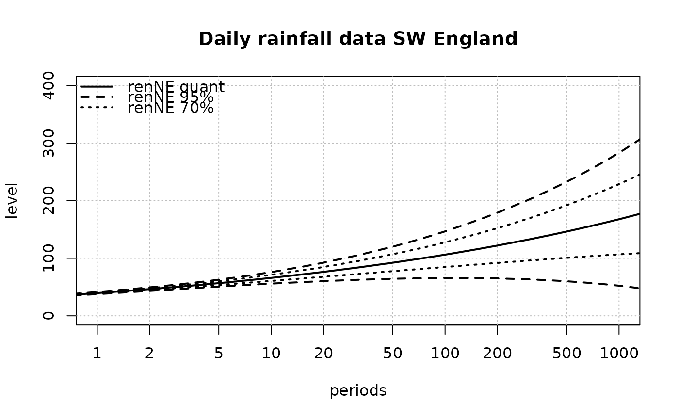
#>    period quant L.95 U.95 L.70 U.70
#> 31     10    66   56   76   61   71
#> 34     20    76   60   92   68   85
#> 36     50    92   64  120   78  107
#> 39    100   106   66  147   85  128
#> 42    200   122   65  179   92  152
#> 43    300   132   63  201   96  169
#> 45    400   140   62  218   99  182
#> 46    500   146   60  233  101  192
#> 47    600   152   58  245  102  201
#> 49    700   156   57  256  104  209
#> 51    800   161   55  266  105  216
#> 52    900   164   54  275  106  223
#> 53   1000   168   52  283  107  229
#> 
#> 
#> o no 'MAX' historical data
#> 
#> o no 'OTS' historical data
#> 
#> o Kolmogorov-Smirnov test
#> NULL
#> 
plot(renNE, main = "Daily rainfall data SW England", ylim = c(0, 400))