Renewal Method for Extreme Values Extrapolation

This package proposes fits and diagnostics for the so-called méthode du renouvellement, an alternative to other "Peaks Over Threshold" (POT) methods. The méthode du renouvellement generalises the classical POT by allowing the excesses over the threshold to follow a probability distribution which can differ from the Generalised Pareto Distribution (GPD). Weibull or gamma excesses are sometimes preferred to GPD excesses. The special case of exponential excesses (which falls in the three families: GPD, Weibull and gamma) has a special interest since it allows exact inference for the (scalar) parameter and for the quantiles form OT data (only).

The package allows the joint use of possibly three kinds of data or information. The first kind is classical excesses, or "OT data". It can be completed with two kinds of data resulting from a temporal aggregation, as is often the case for historical data. Both types are optional, and concern periods or blocks that must not overlap nor cross the OT period.

MAX data correspond to the case where one knows the \(r\) largest observations over each block. The number \(r\) may vary across blocks. This kind of data is often called '\(r\) largest', or "\(r\) Largest Order Statistics" (\(r\) LOS).
OTS data (for OT Supplementary data) correspond to the case where one knows for each block \(b\) all the observations that exceeded a threshold \(u_b\) which is greater (usually much greater) than the main threshold \(u\). The number \(r_b\) of such observations can be zero, in which case we may say that \(u_b\) is an unobserved level. A threshold \(u_b\) is sometimes called a perception threshold.

Historical data are often available in hydrology (e.g. for river flood discharges, for sea-levels or sea surges) and can concern large periods such as past centuries. An unobserved level can typically be related to a material benchmark.

Maximum likelihood estimation is made possible in this context of heterogeneous data. Inference is based on the asymptotic normality of parameter vector estimate and on linearisation ("delta method") for quantiles or parameter functions.

The package allows the use of "marked-process observations" data (datetime of event and level) where an interevent analysis can be useful. It also allows the event dates to be unknown and replaced by a much broader block indication, e.g. a year number. The key point is then that the "effective duration" (total duration of observation periods) is known. Event counts for blocks can be used to check the assumption of Poisson-distributed events.

The package development was initiated, directed and financed by the french Institut de Radioprotection et de Sûreté Nucléaire (IRSN). The package is a non-academic tool designed for applied analysis on case studies and investigations or comparisons on classical probabilistic models.

Details

The DESCRIPTION file: This package was not yet installed at build time.
Index: This package was not yet installed at build time.

This package contains a function Renouv to fit "renouvellement" models.

Author

Yves Deville <deville.yves@alpestat.com>, Lise Bardet <lise.bardet@irsn.fr>

Maintainer: Yann Richet <yann.richet@irsn.fr>

References

Miquel J. (1984) Guide pratique d'estimation des probabilités de crues, Eyrolles (coll. EDF DER).
Coles S. (2001) Introduction to Statistical Modelling of Extremes Values, Springer.
Embrechts P., Klüppelberg C. and Mikosch T. (1997) Modelling Extremal Events for Insurance and Finance. Springer.

Examples

## 'Garonne' data set
summary(Garonne)
#> o Dataset La Garonne river flow
#>    data 'Garonne', variable 'Flow' (m3/s) 
#> 
#> o OT data (main sample) from  1913-01-01  to  1978-01-01  (eff. dur.  65.00 years)
#>  
#>        n     Min.  1st Qu.   Median     Mean  3rd Qu.     Max. 
#>  151.000 2530.000 2900.000 3200.000 3591.675 3995.000 7500.000 
#> 
#> o no missing OT periods 
#> 
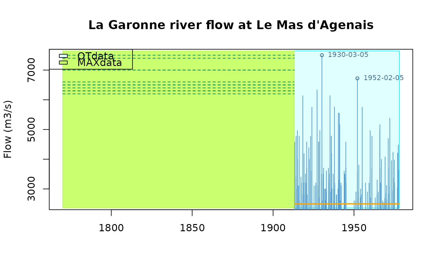
#> o 'MAX' historical info: 1 blocks, 12 obs., total duration = 143.09 years 
#> 
#> o no 'OTS' historical data 
#> 
plot(Garonne)


## Weibull excesses
fG <- Renouv(x = Garonne,
             threshold = 3000,
             distname.y = "weibull",
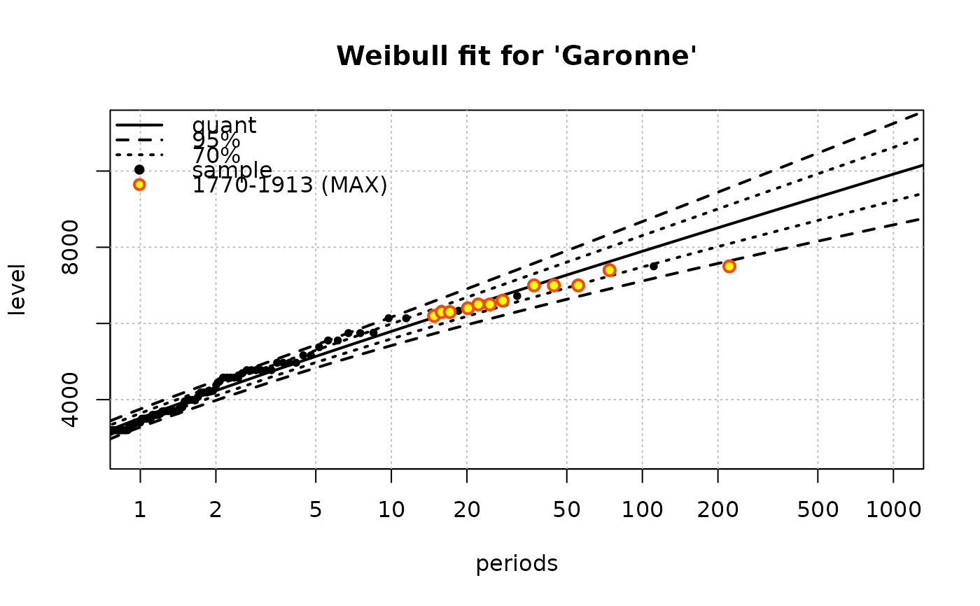
             main = "Weibull fit for 'Garonne'")


coef(fG)
#>      lambda       shape       scale 
#>    1.550137    1.086658 1104.135520 
vcov(fG)
#>               lambda        shape       scale
#> lambda  0.0228075246 0.0007082357   -1.597855
#> shape   0.0007082357 0.0057833653    4.514266
#> scale  -1.5978548466 4.5142657371 8803.576238
summary(fG)
#> o Main sample 'Over Threshold'
#>     . Threshold         3000.00
#>     . Effect. duration    65.00 years
#>     . Nb. of exceed.      98
#> 
#> o Estimated rate 'lambda' for Poisson process (events):  1.55 evt/year.
#> 
#> o Distribution for exceedances y: "weibull", with 2 par. "shape", "scale" 
#> 
#> o No transformation applied
#> 
#> o Coefficients
#> 
#>           Estimate  Std. Error  t value
#> lambda    1.550137  0.15102160 10.26434
#> shape     1.086658  0.07604844 14.28903
#> scale  1104.135520 93.82737467 11.76773
#> 
#> Degrees of freedom: 3 (param.) and 110 (obs)
#> 
#> o Inference method used for return levels
#> "Delta method"
#> 
#> o Return levels
#> 
#>    period quant L.95  U.95 L.70  U.70
#> 28     10  5793 5420  6165 5595  5990
#> 32     20  6436 5964  6909 6187  6686
#> 35     50  7272 6635  7909 6935  7609
#> 37    100  7895 7114  8675 7482  8307
#> 40    200  8510 7574  9446 8015  9005
#> 42    300  8868 7837  9899 8322  9413
#> 44    400  9120 8020 10221 8538  9702
#> 45    500  9315 8160 10471 8704  9926
#> 46    600  9475 8274 10675 8840 10110
#> 48    700  9609 8369 10848 8953 10264
#> 49    800  9725 8451 10998 9051 10398
#> 50    900  9827 8524 11131 9138 10516
#> 51   1000  9919 8588 11249 9215 10622
#> 
#> 
#> o 'MAX' historical info: 1  blocks, 12 obs., total duration = 143.09 years
#> 
#>   * block 1, 143.09 years, 12 obs.
#> 
#>      7500, 7400, 7000, 7000, 7000, 6600, 6500, 6500, 6400, 6300, 6300, 6200
#> 
#> o no 'OTS' historical data
#> 
#> o Kolmogorov-Smirnov test
#> 
#> 	Exact one-sample Kolmogorov-Smirnov test
#> 
#> data:  OTjitter(y.OT, threshold = 0)
#> D = 0.12846, p-value = 0.07196
#> alternative hypothesis: two-sided
#> 
#> 
logLik(fG)
#> [1] -856.4257
#> attr(,"df")
#> [1] 3
#> attr(,"nobs")
#> [1] 110
## Re-plot if needed
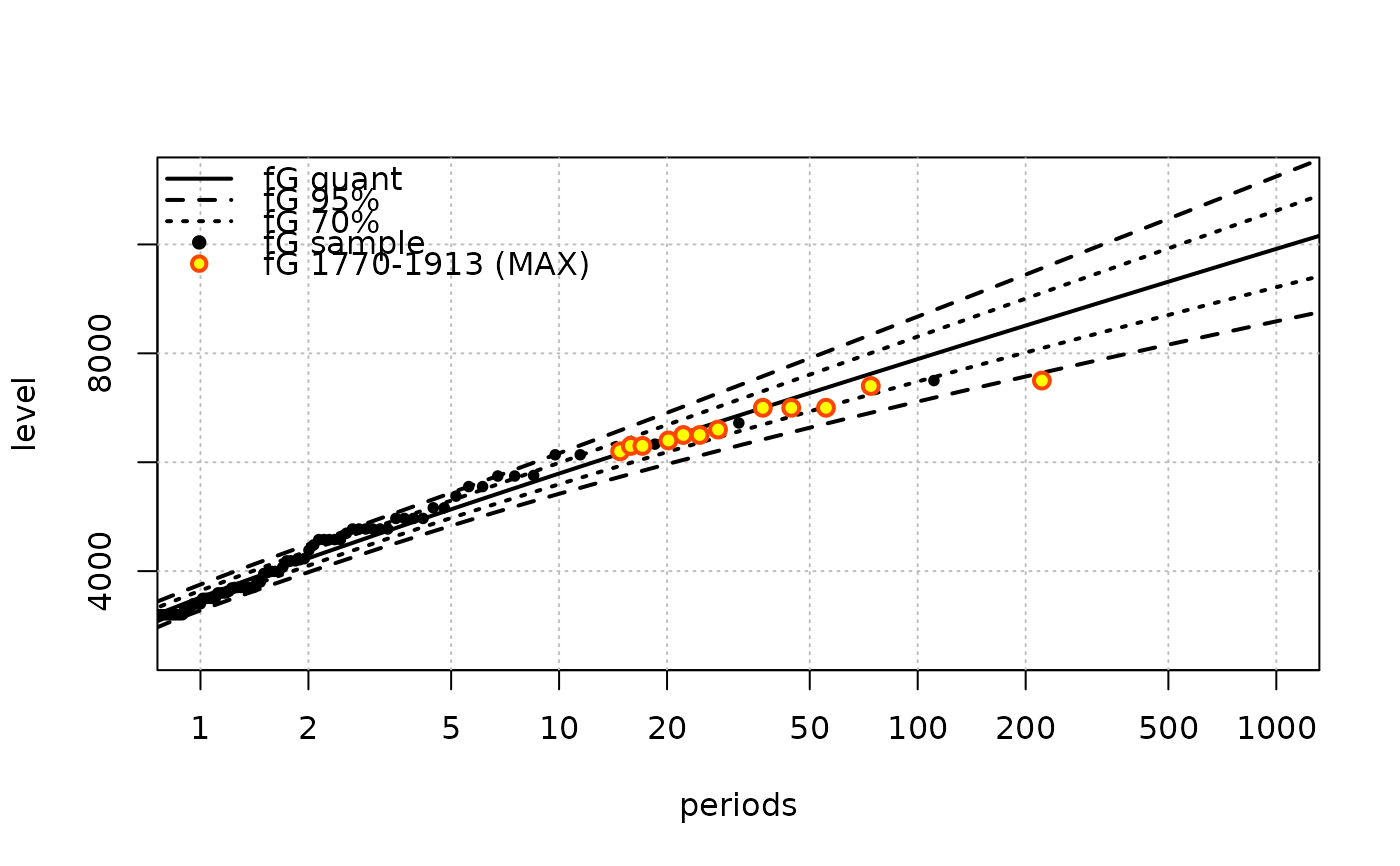
plot(fG)


## Classical 'predict' method with usual formal args 
predict(fG, newdata = c(100, 150, 200), level = c(0.8, 0.9))
#>     period    quant     L.80     U.80     L.90     U.90
#> 100    100 7894.567 7384.096 8405.039 7239.384 8549.751
#> 150    150 8255.550 7686.549 8824.551 7525.245 8985.855
#> 200    200 8510.365 7898.410 9122.319 7724.930 9295.799

Renewal Method for Extreme Values Extrapolation

Details

Author

References

See also

Examples