Mixture of two exponential distributions

Probability functions associated to the mixture of two exponential distributions.

Usage

dmixexp2(x, prob1,
            rate1 = 1.0, rate2 = rate1 + delta, delta,
            log = FALSE)
   pmixexp2(q, prob1,
            rate1 = 1.0, rate2 = rate1 + delta, delta,
            log = FALSE)
   qmixexp2(p, prob1,
            rate1 = 1.0, rate2 = rate1 + delta, delta)
   rmixexp2(n, prob1,
            rate1 = 1.0, rate2 = rate1 + delta, delta)
   hmixexp2(x, prob1,
            rate1 = 1.0, rate2 = rate1 + delta, delta)
   Hmixexp2(x, prob1,
            rate1 = 1.0, rate2 = rate1 + delta, delta)

Arguments

x, q

Vector of quantiles.

p

Vector of probabilities.

n

Number of observations.

log

Logical; if TRUE, the log density is returned.

prob1

Probability weight for the "number 1" exponential density.

rate1

Rate (inverse expectation) for the "number 1" exponential density.

rate2

Rate (inverse expectation) for the "number 2" exponential density. Should in most cases be > rate1. See Details.

delta

Alternative parameterisation delta = rate2 - rate1.

Value

dmiwexp2, pmiwexp2, qmiwexp2, evaluates the density, the distribution and the quantile functions. dmixexp2

generates a vector of n random draws from the distribution.

hmixep2 gives hazard rate and Hmixexp2 gives cumulative hazard.

Details

The density function is the mixture of two exponential densities $$ f(x) = \alpha_1 \lambda_1 \, e^{-\lambda_1 x} + (1-\alpha_1) \lambda_2 \, e^{-\lambda_2x} \qquad x > 0 $$ where \(\alpha_1\) is the probability given in prob1 while \(\lambda_1\) and\(\lambda_2\) are the two rates given in rate1 and rate2.

A 'naive' identifiability constraint is $$\lambda_1 < \lambda_2$$ i.e. rate1 < rate2, corresponding to the simple constraint delta > 0. The parameter delta can be given instead of rate2.

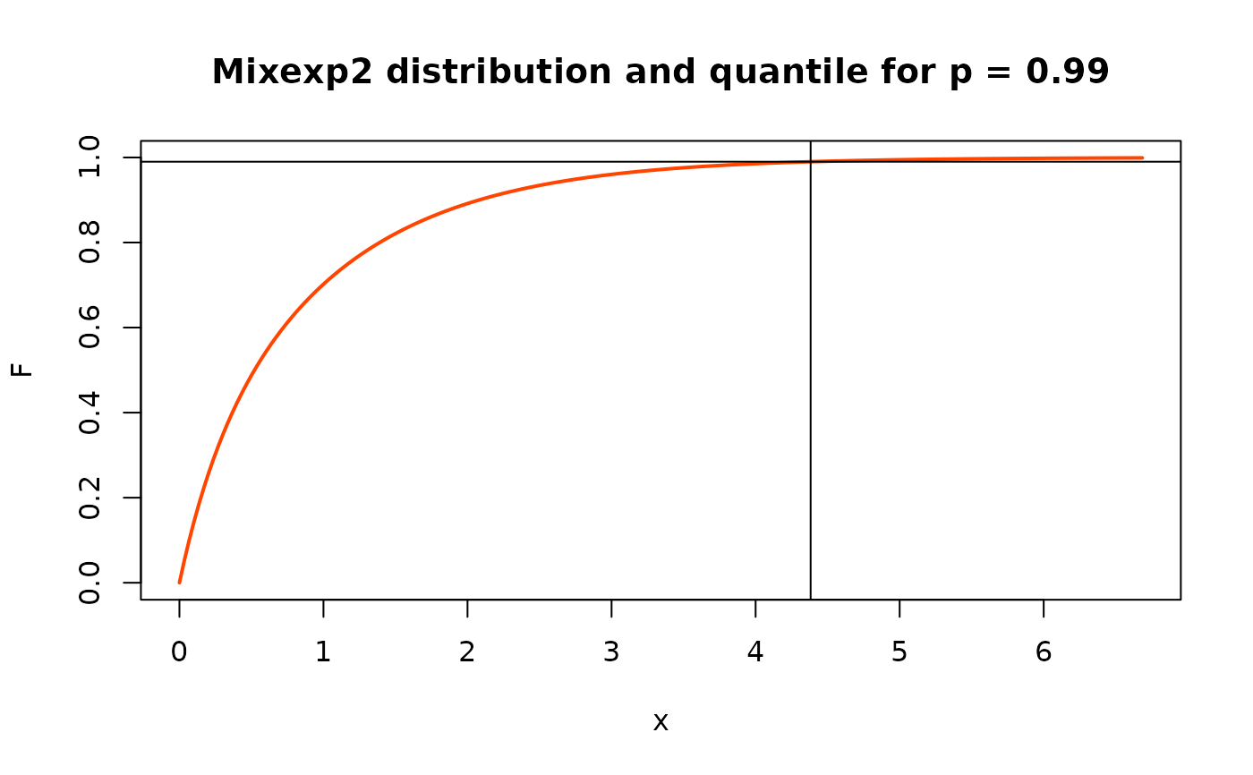
The mixture distribution has a decreasing hazard, increasing Mean Residual Life (MRL) and has a thicker tail than the usual exponential. However the hazard, MRL have a finite non zero limit and the distribution behaves as an exponential for large return levels/periods.

The quantile function is not available in closed form and is computed using a dedicated numerical method.

Examples

rate1 <- 1.0
rate2 <- 4.0
prob1 <- 0.8
qs <- qmixexp2(p = c(0.99, 0.999), prob1 = prob1,
               rate1 = rate1, rate2 = rate2) 
x <- seq(from = 0, to = qs[2], length.out = 200)
F <- pmixexp2(x, prob1 = prob1, rate1 = rate1, rate2 = rate2)
plot(x, F, type = "l", col = "orangered", lwd = 2,
     main = "Mixexp2 distribution and quantile for p = 0.99")
abline(v = qs[1])
abline(h = 0.99)